Week 07 · Learning from Evidence: Likelihood, Bayesian Inference, and Latent Variables
English · Русский
A rain indicator can make mistakes, and repeated measurements can differ. How can observations help us understand these errors and fit better predictions? We need to distinguish a recorded outcome from a model of the outcomes that could occur.
Earlier chapters used mean squared error and cross-entropy to train predictions. Why those losses? A probability model provides an answer: specify the possible observations and how their probabilities depend on the model, then ask which parameters best explain the data. A further question follows: what uncertainty remains after fitting?
The chapter connects likelihood-based losses to Bayesian parameter inference and, finally, inference about an image’s hidden code. Each objective follows from an observation model, a prior, or an explicitly stated approximation.
Learning outcomes:
- distinguish probability mass, density, likelihood, and posterior uncertainty;
- derive classification and regression losses from stated observation models;
- explain when evidence can be treated as constant and how a Gaussian prior gives an L2 penalty;
- distinguish parameter uncertainty from observation noise; and
- explain the inference roles of dropout and a variational autoencoder (VAE).
Prerequisites and companions. We assume basic algebra and the Week 04 learning loop; later derivations use calculus and matrix multiplication. The Week 07 lecture supplies the visual overview. The tutorial develops Bayesian regression, dropout, and a small VAE through executable experiments.
Notation. Capital letters such as \(R,S,X,Y\) denote random variables; lowercase letters denote their possible or recorded values. We use \(p(y)\) for a mass or density, with its kind stated beside it. An event is a set of outcomes. We write \(P(A)\) for the probability of an event \(A\) and identify whether a function \(p\) is a probability mass function or a density.
| Symbol | Meaning in this chapter |
|---|---|
| \(R,S\); \(\rho\) | Binary rain and sensor variables; a Bernoulli success probability |
| \(\mu,\sigma^2\) | Mean and variance of the distribution currently being discussed |
| \(\mathbb E\), \(\operatorname{Var}\) | Expectation and variance, with the averaging distribution stated |
| \(\mathcal D=\{(x_i,y_i)\}_{i=1}^n\), \(\theta\) | Observed input–target pairs (\(n\) examples, indexed by \(i\)) and model parameters |
| \(\Lambda(\theta;\mathcal D)\) | Likelihood: fixed observations, variable candidate parameters |
| \(L_i\), \(L=\sum_i L_i\), \(\bar L=L/n\) | Per-observation, summed, and mean loss |
We retain the course’s \(\phi\) for an activation and \(L\) for loss; earlier chapters also used \(\mathcal L\) for particular objectives. Writing \(p(y\mid x,\theta)\) makes the given parameters explicit; it does not assume that they are random. A posterior over parameters will be introduced separately. A hat marks an estimate or prediction; a bar marks an average. The symbols \(\sum\) and \(\prod\) mean sum and product over the indicated index. Logs \(\ln\) are natural logarithms; \(\exp(a)=e^a\). Specialized symbols and tensor shapes will be introduced where their calculations begin. In particular, a predicted probability and a predicted real-valued mean will be named separately.
Probability describes what we do not know
Allow about 15 minutes for this recap. We will turn counts into probability rules, distinguish mass from density, and summarize a distribution by its mean and variance (Bishop 2006, secs. 1.2–1.2.2).
Rain and a sensor: joint, marginal, conditional, and Bayes
Imagine a device that signals rain. It sometimes signals on a dry day and sometimes misses rain. Recording its indication alongside the weather lets us examine these mistakes: how often does it signal when rain occurs, and how much should a signal change our belief about rain?
Let \(R=1\) mean rain and \(S=1\) a signal; zero means dry or no signal. For comparison with the lecture, write \(Y=R\), \(X=S\). The following synthetic table records both on the same day.
|
Weather Y = R |
No signal X = S = 0 |
Signal X = S = 1 |
Row total |
|---|---|---|---|
|
Dry Y = 0 |
54\(n_{00}\) | 6\(n_{01}\) | 60\(r_0\) |
|
Rain Y = 1 |
16\(n_{10}\) | 24\(n_{11}\) · rain + signal | 40\(r_1\) |
| Column total | 70\(c_0\) | 30\(c_1\) | 100\(N\) |
Weather marginal: \(p(y=0)=r_0/N=0.60\);
\(p(y=1)=r_1/N=0.40\).
Signal marginal: \(p(x=0)=c_0/N=0.70\);
\(p(x=1)=c_1/N=0.30\).
Imagine choosing one recorded day uniformly. A fraction is then an exact probability for this finite model; estimating population probabilities from a sample needs additional assumptions. The table does not establish independent days or real forecast performance.
The joint probability specifies both outcomes: \(p(y_i,x_j)=n_{ij}/N\). Adding cells removes one variable: \(p(x_j)=\sum_i p(y_i,x_j)=c_j/N\). This is marginalization, or the sum rule. Here subscripts \(i,j\) label table categories; later \(i\) will index dataset observations.
The vertical bar in \(p(y_i\mid x_j)\) means “given”: restrict attention to days with signal value \(x_j\). Among those \(c_j\) days, \(n_{ij}\) have weather value \(y_i\). Thus the conditional probability is \(n_{ij}/c_j\), provided \(c_j>0\). Multiply by the probability of that reference group:
\[ \underbrace{p(y_i\mid x_j)}_{n_{ij}/c_j} \underbrace{p(x_j)}_{c_j/N} =\frac{n_{ij}}{N}=p(y_i,x_j). \]
This cancellation explains the product rule. Restricting to a weather row instead gives \(p(x_j\mid y_i)=n_{ij}/r_i\). Equate the two factorizations of the same joint and divide by positive \(p(x_j)\):
\[ p(y_i\mid x_j)=\frac{p(x_j\mid y_i)p(y_i)}{p(x_j)}. \]
Bayes’ rule updates information. Before knowing the signal, rain has probability \(0.4\) (the prior). A signal is observed; its probability given rain is \(24/40=0.6\). The total probability of a signal is
\[ p(x=1)=0.6(0.4)+0.1(0.6)=0.3, \]
summing the rainy and dry routes. The updated rain probability (the posterior) is \(0.6(0.4)/0.3=0.8=24/30\). Knowing the signal changes which days we count. The update concerns available information; it need not describe events occurring in that order. Signal-given-rain (\(0.6\)) and rain-given-signal (\(0.8\)) answer different questions.
Independence would require \(p(x,y)=p(x)p(y)\) for every pair; here \(0.24\ne0.3(0.4)\). Mutually exclusive events instead cannot occur together. Rain and a signal can.
Probability mass and density describe different kinds of outcomes
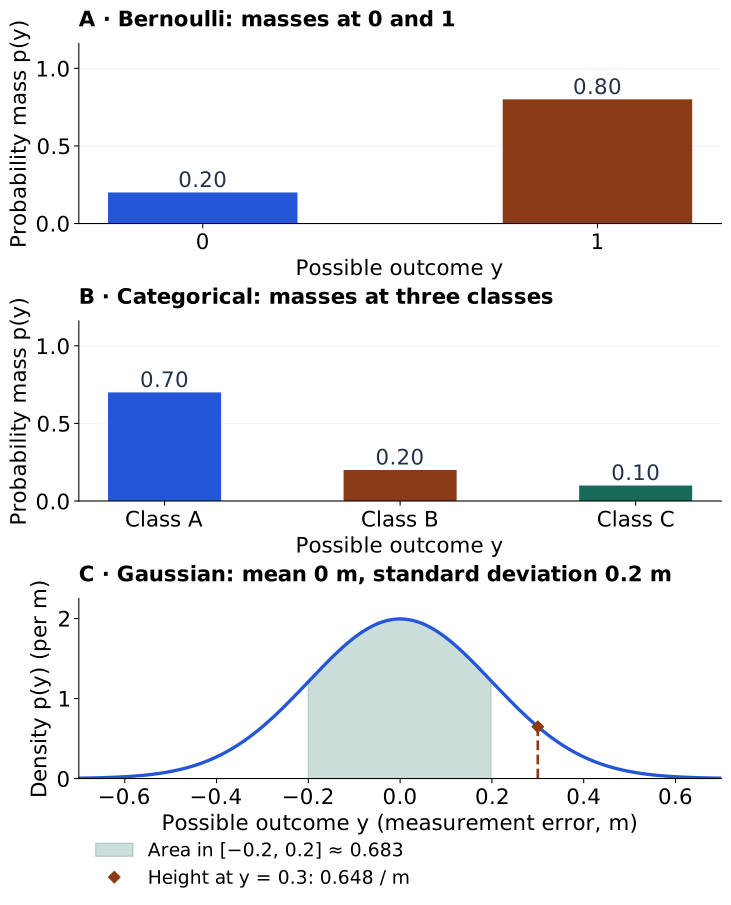
A probability mass function (PMF) assigns a probability \(p(y)\) to each discrete outcome, with \(p(y)\ge0\) and \(\sum_y p(y)=1\). A Bernoulli distribution has outcomes 0 and 1, with masses \(1-\rho\) and \(\rho\). A categorical distribution assigns masses to \(C\) mutually exclusive classes; its probability vector sums to one.
Figure 1 compares these with a continuous normal, or Gaussian, distribution. Its probability density function (PDF), parameterized by mean \(\mu\), variance \(\sigma^2>0\), and standard deviation (SD) \(\sigma=\sqrt{\sigma^2}\), is
\[ p(y)=\frac{1}{\sqrt{2\pi}\,\sigma} \exp\!\left[-\frac{(y-\mu)^2}{2\sigma^2}\right]. \]
We also write \(Y\sim\mathcal N(\mu,\sigma^2)\): \(\sim\) means “is distributed as,” and \(\mathcal N\) denotes a Gaussian with the given mean and variance. Integrals without limits run over the variable’s full domain. Density is nonnegative and integrates to one. For interval endpoints \(a\le b\), area gives probability:
\[ \int p(y)\,dy=1,\qquad P(a\le Y\le b)=\int_a^b p(y)\,dy. \]
The Gaussian peak is about \(1.995\) per metre; the shaded interval has probability \(0.683\). Density can exceed one and has inverse measurement units. An exact point has zero probability in this continuous model; a rounded reading represents an interval. Later, a network will supply these families’ parameters for each input.
The same rules, now for densities. For a normalized joint model,
\[ p(x,y)=p(y\mid x)p(x)=p(x\mid y)p(y). \]
Bayes gives \(p(y\mid x)=p(x\mid y)p(y)/p(x)\) for positive finite \(p(x)\). Hold \(x\) fixed and integrate over possible \(y\). Since a conditional density integrates to one,
\[ \begin{aligned} p(x)&=p(x)\underbrace{\int p(y\mid x)\,dy}_{1}\\ &=\int p(x\mid y)p(y)\,dy\\ &=\int p(x,y)\,dy. \end{aligned} \]
The denominator is the joint model with \(y\) removed—the continuous version of adding table cells. For discrete \(y\), use a sum. This recovers marginalization from the same normalized joint; a conditional density is not a ratio of zero-probability point events.
Expectation and variance summarize a distribution
For a numerical outcome \(Y\), expectation weights possible values by their mass or density. Assuming the first moment exists,
\[ \begin{aligned} \mu=\mathbb E[Y]&=\sum_y y\,p(y) &&\text{(discrete)},\\ \mu=\mathbb E[Y]&=\int y\,p(y)\,dy &&\text{(continuous)}. \end{aligned} \]
With a finite second moment, variance averages squared deviations:
\[ \begin{aligned} \operatorname{Var}(Y)&=\sum_y(y-\mu)^2p(y) &&\text{(discrete)},\\ \operatorname{Var}(Y)&=\int(y-\mu)^2p(y)\,dy &&\text{(continuous)}. \end{aligned} \]
Expanding the square gives \(\mathbb E[Y^2]-2\mu\mathbb E[Y]+\mu^2=\mathbb E[Y^2]-\mu^2\). For Bernoulli outcomes, \(\mathbb E[Y]=0(1-\rho)+1\rho=\rho\) and \(Y^2=Y\), hence \(\operatorname{Var}(Y)=\rho(1-\rho)\). A mean of \(0.8\) need not be a possible observation. Arbitrary categorical class IDs have no meaningful numerical mean.
In the Gaussian panel, the mean is \(0\) m, variance \(0.04\) m², and standard deviation \(\sqrt{\operatorname{Var}(Y)}=0.2\) m. A model expectation averages possible outcomes; the sample mean \(n^{-1}\sum_i y_i\) averages recorded observations.
Pause. Which heights in the figure are probabilities? Which require an area? What must a network output to specify each distribution? Next we fix observations and vary candidate model parameters to define a likelihood.
From an observed dataset to a training objective
A dataset contains observations; a probability model describes how observations could arise. Fitting connects them by asking which parameters assign the observed data the largest likelihood (Bishop 2006, sec. 1.2.5).
The joint probability comes before the independence assumption
Repeatedly apply the two-variable product rule to obtain the chain rule for arbitrary quantities \(x_1,\ldots,x_n\):
\[ p(x_1,\ldots,x_n) =p(x_1)\prod_{k=2}^n p(x_k\mid x_1,\ldots,x_{k-1}). \]
Here the \(x_k\) are generic quantities; the formula does not assume independent features. Apply the same rule to the joint mass or density of \(n\) input–target pairs:
\[ \begin{aligned} p(x_{1:n},y_{1:n}\mid \theta) &=p(x_1,y_1\mid \theta)\\ &\quad\times\prod_{i=2}^n p(x_i,y_i\mid x_{1:i-1},y_{1:i-1},\theta). \end{aligned} \]
Here \(x_{1:n}=(x_1,\ldots,x_n)\), and similarly for targets. No independence has been assumed. If the pairs are independent, earlier pairs can be removed from each conditioning set. If they are also identically distributed, one shared sampling law describes every pair. These are the iid assumptions. They give
\[ \begin{aligned} p(x_{1:n},y_{1:n}\mid \theta) &=\prod_{i=1}^n p(x_i,y_i\mid \theta)\\ &=\prod_{i=1}^n p(y_i\mid x_i,\theta)p(x_i\mid \theta). \end{aligned} \]
Independence concerns different pairs; it does not make an input independent of its own target. Repeated measurements from one subject or neighboring time steps may violate it.
In supervised prediction we usually specify a conditional model directly, holding observed inputs fixed. Under the conditional factorization above,
\[ p(y_{1:n}\mid x_{1:n},\theta)=\prod_{i=1}^n p(y_i\mid x_i,\theta). \]
This can also be a modeling assumption for fixed experimental inputs, without modeling their distribution. A shared rule need not give identical target distributions at different inputs: a sensor’s expected reading can depend on \(x_i\). Starting from a joint objective, omitting its input factor preserves the optimization only when that factor is independent of fitted parameters. Merely observing the inputs does not establish that condition.
Maximum likelihood and negative log likelihood
Define the likelihood \(\Lambda(\theta;\mathcal D)=p(y_{1:n}\mid x_{1:n},\theta)\). The observations stay fixed while candidate parameters vary. It scores explanations of those data; it is not a normalized probability distribution over \(\theta\).
Maximum likelihood estimation (MLE) chooses maximizing parameters. Here \(\arg\max\) returns parameter settings that maximize an expression; \(\arg\min\) returns those that minimize it. The symbol \(\in\) means “is one of.” For positive likelihood, the logarithm is strictly increasing, so the following objectives select the same maximizers/minimizers:
\[ \begin{aligned} \widehat\theta_{\mathrm{MLE}} &\in\arg\max_\theta\Lambda(\theta;\mathcal D)\\ &=\arg\max_\theta\sum_{i=1}^n\ln p(y_i\mid x_i,\theta)\\ &=\arg\min_\theta\left[-\sum_{i=1}^n\ln p(y_i\mid x_i,\theta)\right]. \end{aligned} \]
The notation selects any optimizer when several exist. Logarithms turn products into sums; the negative sign turns maximization into minimization. This negative log likelihood (NLL) is \(L=\sum_i L_i\), where \(L_i=-\ln p(y_i\mid x_i,\theta)\). Computing log scores directly also avoids underflow from multiplying many tiny probabilities. The mean \(\bar L=L/n\) has the same unregularized minimizers, but gradients are divided by \(n\). Natural-log scores use nats.
For a separate synthetic ordered sequence \((1,0,0,1,0,0,0,1,0,0)\), assume iid Bernoulli observations with constant rain probability \(\rho\). Three rain events and seven dry events give
\[ \Lambda(\rho)=\rho^3(1-\rho)^7,\qquad \frac{d\ln\Lambda}{d\rho}=\frac3\rho-\frac7{1-\rho}. \]
Setting the derivative to zero gives \(\widehat\rho=3/10\); the log likelihood is strictly concave on \((0,1)\) and the likelihood vanishes at both endpoints. This sequence is distinct from the earlier 100-day table. Observing only the count instead gives \(\binom{10}{3}\rho^3(1-\rho)^7\): the binomial coefficient \(\binom{10}{3}=120\) counts the sequences with three ones. This parameter-independent factor leaves the MLE unchanged.
MLE is a central frequentist estimation method. In that interpretation parameters are fixed unknown quantities; estimates vary across hypothetical repeated datasets. Frequentist statistics includes other estimators and uncertainty procedures. Bayesian inference also uses likelihoods; it combines them with a prior later in this chapter.
Classification losses follow from discrete observation models
Return to the discrete panels in Figure 1. We choose a distribution family; the network supplies its parameters for each input. The distribution describes possible targets, and the observed target selects the mass to score. Taking its negative log produces the loss (Bishop 2006, secs. 2.1–2.2).
Bernoulli: from two cases to binary cross-entropy
For a binary target, the network maps input \(x_i\) to a scalar logit \(z_i\), using trainable parameters \(\theta\). A sigmoid turns this logit into the Bernoulli success probability:
\[ \widehat y_i=\operatorname{sigmoid}(z_i) =\frac{1}{1+e^{-z_i}} =P(y_i=1\mid x_i,\theta). \]
Here \(P(y_i=1\mid x_i,\theta)\) denotes the probability of label one for this input and these weights, before looking at its recorded label. The scalar \(\widehat y_i\) specifies both masses, \(1-\widehat y_i\) and \(\widehat y_i\). It is a distribution parameter; \(y_i\) is the recorded label. In Figure 2, follow the network output to the distribution and then to the observed-label score.
Parameters θ determine the network logit zᵢ. The observed label yᵢ is not a network input. One scalar ŷᵢ specifies both bars.
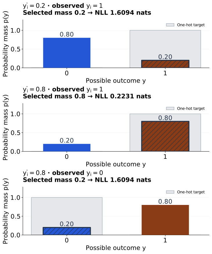
Pale gray: one-hot target (0, 1). Colored bars: model probabilities.
The sweep compares candidate predictions at a fixed input xᵢ; it is not a training trace. Changing yᵢ selects a different illustrative observation. Hatching and ▲ mark the selected outcome.
Reduced motion is enabled: use the slider or probability buttons to compare states.
Write the selection first as two instructions: if \(y_i=1\), return \(\widehat y_i\); if \(y_i=0\), return \(1-\widehat y_i\). A piecewise PMF and an exponent selector express those same instructions:
\[ \begin{aligned} p(y_i\mid x_i,\theta) &=\begin{cases} \widehat y_i,&y_i=1,\\ 1-\widehat y_i,&y_i=0 \end{cases}\\ &=\widehat y_i^{\,y_i}(1-\widehat y_i)^{1-y_i}. \end{aligned} \]
For label one the exponents \((1,0)\) select \(\widehat y_i\); for label zero, \((0,1)\) select \(1-\widehat y_i\). Under conditional independence, substitute this PMF into the dataset product and take its negative log:
\[ \begin{aligned} \Lambda(\theta;\mathcal D) &=\prod_i\widehat y_i^{\,y_i}(1-\widehat y_i)^{1-y_i},\\ L_{\mathrm{BCE}}(\theta) &=-\sum_i\left[y_i\ln\widehat y_i +(1-y_i)\ln(1-\widehat y_i)\right]. \end{aligned} \]
This is summed binary cross-entropy (BCE); divide by \(n\) for the mean. At \(\widehat y_i=0.8\), label one costs \(0.2231\) nats, label zero \(1.6094\) nats. The algebra uses \(0<\widehat y_i<1\); endpoint losses are limits. Zero mass on the observed label gives infinite loss; mass one gives zero. A thresholded class decision is a separate operation.
Categorical: from one observed class to cross-entropy
When exactly one of \(C\) classes is observed, the output head supplies \(C\) logits, \(z_{i,c}\), for \(c=0,\ldots,C-1\). Write \(z_i=(z_{i,0},\ldots,z_{i,C-1})\) for their vector. Softmax converts them to a probability vector; \(j\) in its denominator is another class index being summed over:
\[ \widehat y_{i,c}=\frac{e^{z_{i,c}}}{\sum_{j=0}^{C-1}e^{z_{i,j}}}, \qquad \sum_c\widehat y_{i,c}=1. \]
Figure 3 follows the same route with three masses. Define a one-hot target, \(y^{\mathrm{one\text{-}hot}}_{i,c}=1\) when \(y_i=c\) and zero otherwise. Exactly one entry is one. Thus
\[ p(y_i\mid x_i,\theta) =\prod_c\widehat y_{i,c}^{\,y^{\mathrm{one\text{-}hot}}_{i,c}} =\widehat y_{i,y_i}. \]
The product selects one mass; it does not assert independence between mutually exclusive class indicators. Multiply across conditionally independent examples, then take negative logs:
\[ \begin{aligned} \Lambda(\theta;\mathcal D) &=\prod_i\prod_c\widehat y_{i,c}^{\,y^{\mathrm{one\text{-}hot}}_{i,c}},\\ L_{\mathrm{CE}} &=-\sum_i\sum_c y^{\mathrm{one\text{-}hot}}_{i,c}\ln\widehat y_{i,c}\\ &=-\sum_i\ln\widehat y_{i,y_i}. \end{aligned} \]
zᵢ,₁
zᵢ,₂
Three predictions and three observed one-hot values enter the observation model; the target is used for scoring, not fed into the network.
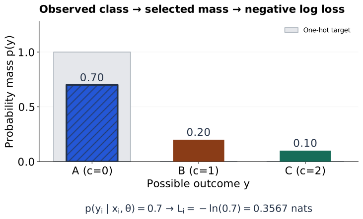
Divide by \(n\) for mean CE. Other class probabilities enter through Softmax normalization. Multiple simultaneous labels instead need binary observation models, commonly one Bernoulli term per label.
Cross-entropy scores one distribution with another: \(H(q,p)=-\sum_c q_c\ln p_c\). Here \(q\) is the observed one-hot distribution and \(p\) is the prediction; averaging over observations gives empirical mean cross-entropy. BCE applies the same definition to two outcomes.
Use fused losses directly on logits for stability (PyTorch contributors, n.d.-a, n.d.-b). This CPU example uses batch size \(B=2\):
import torch
from torch.nn import functional as F

# Binary: logits and floating targets both have shape (B, 1).
z_binary = torch.tensor([[1.3862944], [1.3862944]])
y_binary = torch.tensor([[1.0], [0.0]])
bce = F.binary_cross_entropy_with_logits(
    z_binary, y_binary, reduction="mean"
)

# Categorical: logits (B, C); integer class indices (B,).
z_class = torch.tensor([[2.0, 0.0, -1.0], [0.0, 1.0, 2.0]])
y_class = torch.tensor([0, 2], dtype=torch.long)
ce = F.cross_entropy(z_class, y_class, reduction="mean")
assert bce.ndim == ce.ndim == 0
The binary logit is approximately \(\ln4\), giving probability \(0.8\). These unweighted losses average two examples. One-hot notation explains the algebra; this categorical code uses integer targets. Do not apply sigmoid or Softmax before the fused losses: they implement those transformations internally. Gaussian regression, developed next, starts with a density and yields Gaussian NLL or scaled squared error.
Regression losses follow from Gaussian observation models
For real-valued targets, the network can supply a Gaussian’s mean instead of class probabilities. The same likelihood recipe now produces squared error—and tells us when squared error alone is insufficient (Bishop 2006, sec. 1.2.5).
A conditional density at one input
The tutorial generates readings using \(y=0.3+2x+\epsilon\), with \(\epsilon\sim\mathcal N(0,0.25^2)\). That generator is known in a teaching experiment; a fitted model must estimate an unknown mean function \(\mu(x;\theta)\). The semicolon separates input \(x\) from fitted parameters \(\theta\). A Gaussian noise law is a modelling assumption, not a consequence of taking many observations.
The mean head supplies a real-valued network output \(z_i\), with identity output transformation: \(\widehat y_i=z_i=\mu(x_i;\theta)\). Unlike a classification logit, this output directly represents a mean. This is an expected reading, so its meaning differs from a classification probability. With fixed standard deviation \(\sigma\), it specifies
\[ p(y\mid x_i,\theta)=\frac1{\sqrt{2\pi}\,\sigma} \exp\!\left[-\frac{(y-\widehat y_i)^2}{2\sigma^2}\right]. \]
Here \(y\) ranges over possible readings; the recorded \(y_i\) selects one density height. In Figure 4, choose an observation, then move the candidate mean. The left panel fixes an input with a vertical guide; the right displays the possible target values along that slice, turned onto a horizontal axis. Both refer to the same observation.
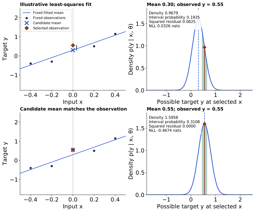
● fixed observations · ◆ selected yᵢ · × candidate mean · dashed blue: mean · green area: interval probability. The right panel displays the target values along the left panel’s vertical guide.
Choosing an observation resets the offset to the fitted mean. The mean sweep holds that observation and σ fixed. It compares local predictions; it is not a training trace or a new globally fitted curve. The isolated cross may move away from the fixed fitted line.
Reduced motion is enabled: use the slider and comparison buttons.
The initial selected point is \((0,0.55)\); the fitted mean is \(0.30\), with \(\sigma=0.25\). Its density is about \(0.9679\), and the probability of a reading in \([0.45,0.65]\) is about \(0.1935\). Moving the mean to \(0.55\) raises these to \(1.5958\) and \(0.3108\). The point itself still has zero probability in this continuous model. Unlike a discrete mass, density can exceed one, so Gaussian NLL can be negative. Its numerical value depends on the target’s measurement units.
For conditionally independent observations, form the dataset likelihood and take its negative log:
\[ \Lambda(\theta;\mathcal D)=\prod_i p(y_i\mid x_i,\theta), \qquad L=-\ln\Lambda=\sum_i L_i. \]
Write \(\sigma_i^2\) to allow a different variance at each input. The Gaussian’s normalization and exponential terms give
\[ \begin{aligned} L_i&=-\ln p(y_i\mid x_i,\theta)\\ &=\frac{(y_i-\widehat y_i)^2}{2\sigma_i^2} +\frac12\ln\sigma_i^2+\frac12\ln(2\pi). \end{aligned} \]
The quadratic term comes directly from the Gaussian exponent. The log-variance term comes from its normalization; it is part of the same observation model.
Common variance gives scaled squared error
Homoscedastic means the observation variance is the same at every input: \(\sigma_i^2=\sigma^2\). If that common variance is fixed while fitting the mean, averaging gives
\[ \begin{aligned} \operatorname{MSE}&=\frac1n\sum_i(y_i-\widehat y_i)^2,\\ \bar L&=\frac{\operatorname{MSE}}{2\sigma^2} +\frac12\ln\sigma^2+\frac12\ln(2\pi). \end{aligned} \]
The last two terms are constant in \(\theta\), and \(1/(2\sigma^2)>0\). Minimizing mean NLL therefore gives the same fitted mean as minimizing MSE, although the objective values and gradient scales differ. Fixed unequal variances instead give weighted squared error, with weight \(1/\sigma_i^2\).
Common variance need not be known. If we learn it, retain its log term. For fixed fitted means and positive MSE, differentiating the mean NLL with respect to \(v=\sigma^2\) gives
\[ \frac{\partial\bar L}{\partial v} =-\frac{\operatorname{MSE}}{2v^2}+\frac1{2v}=0 \quad\Longrightarrow\quad \widehat{\sigma^2}_{\mathrm{MLE}}=\operatorname{MSE}. \]
This is a likelihood estimate, not the degrees-of-freedom-corrected residual variance. If every residual vanishes, no positive unconstrained variance maximizes likelihood: it increases without bound as variance approaches zero.
Input-dependent variance gives a heteroscedastic loss
Heteroscedastic means observation variance depends on the input. Add a variance output head alongside the mean head. The two heads predict a mean and a log variance:
\[ x_i\longrightarrow\text{network} \longrightarrow \begin{cases} \widehat y_i=\mu(x_i;\theta),\\ s_i=s(x_i;\theta),\quad \sigma_i^2=e^{s_i}>0. \end{cases} \]
Both are distribution parameters; neither is a sampled target. Substituting into the Gaussian NLL gives
\[ L_i=\frac12\left[e^{-s_i}(y_i-\widehat y_i)^2+s_i+\ln(2\pi)\right]. \]
Increasing variance reduces the residual’s weight, but also increases the log-variance cost. Omitting \(s_i\) would let the model reduce the loss merely by inflating variance. For fixed mean,
\[ \frac{\partial L_i}{\partial s_i} =\frac12\left[1-e^{-s_i}(y_i-\widehat y_i)^2\right]. \]
For nonzero residual, this balances at variance equal to its square; a shared network generally cannot choose each example’s variance independently. At an exact fit, unrestricted variance can collapse. A positive variance floor can prevent that degeneracy: for example, use \(\sigma_i^2=\sigma_{\min}^2+\operatorname{softplus}(v_i)\) and evaluate the NLL with this actual variance. Here \(\sigma_{\min}>0\) is a chosen minimum SD, \(\operatorname{softplus}(v)=\ln(1+e^v)\), and \(v_i\) is an unconstrained head output, not its log variance.
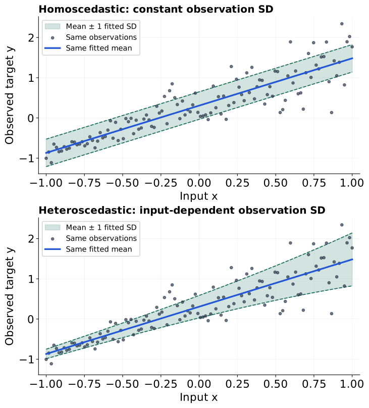
Figure 5 makes this difference visible on data with increasing noise. Both panels keep the same least-squares mean to isolate the spread: minimizing Gaussian NLL fits a common SD in the upper panel, and a log variance linear in \(x\) in the lower panel. The variable-width band better describes this dataset’s changing scatter; it need not improve the mean curve or MSE. In a network, the additional variance head learns that input-to-spread mapping, usually jointly with the mean head. Predicted spread describes observation noise conditional on fitted weights; it does not by itself represent uncertainty about those weights. In code, target, mean and per-input variance arrays should have matching shape, such as \((B,1)\), to avoid unintended broadcasting. Sum the per-observation terms, or declare their mean reduction.
The route from observation model to loss is now the same in all three cases:
| Target support | Model output | Per-observation NLL |
|---|---|---|
| Binary \(\{0,1\}\) | Sigmoid probability \(\widehat y_i\) | BCE |
| One of \(C\) classes | Softmax vector \(\widehat y_{i,c}\) | Categorical CE |
| Real-valued | Mean; fixed common variance | Scaled squared error + constant |
| Real-valued | Mean and input-dependent variance | Gaussian NLL with log-variance term |
The remaining modelling choice is what to retain after fitting: one set of weights, or a distribution over plausible weights. That leads to Bayesian learning.
Bayesian learning updates a distribution over unknowns
The same data can support several plausible parameter settings. Bayesian learning represents that uncertainty with a distribution over parameters, then updates it using the likelihood. A point estimate can still be useful; keeping it is a further choice (Bishop 2006, secs. 1.2.3–1.2.6).
Prior, likelihood, posterior, and evidence
Fix observed inputs \(X=(x_1,\ldots,x_n)\) and targets \(\mathbf y=(y_1,\ldots,y_n)\). Choose a conditional model and a proper prior \(p(\theta)\): a normalized distribution expressing assumptions about parameters before using these targets. The likelihood \(p(\mathbf y\mid X,\theta)\) is the one already used for BCE, CE or Gaussian regression. Bayes’ rule gives
\[ \underbrace{p(\theta\mid\mathcal D)}_{\text{posterior}} =\frac{\overbrace{p(\mathbf y\mid X,\theta)}^{\text{likelihood}} \overbrace{p(\theta)}^{\text{prior}}} {\underbrace{p(\mathbf y\mid X)}_{\text{evidence}}}. \]
The evidence totals the data’s likelihood over all parameter settings, weighted by their prior density:
\[ p(\mathbf y\mid X) =\int p(\mathbf y\mid X,\vartheta)p(\vartheta)\,d\vartheta. \]
Here \(\vartheta\) is a dummy integration variable for the whole parameter vector. Assume the evidence is positive and finite. Dividing by it normalizes the posterior. The posterior can retain spread or several modes; drawing from it explores plausible settings. Gradient updates instead move a fitted setting. We need not suppose that the physical system redraws its weights for each measurement.
When is the evidence a constant?
Constant means independent of the variable currently being varied. With data, model and prior settings fixed, the evidence integral has already eliminated the candidate \(\theta\). Consequently,
\[ p(\theta\mid\mathcal D)\propto p(\mathbf y\mid X,\theta)p(\theta). \]
The symbol \(\propto\) means “proportional to,” with one common normalizer. This is a consequence of the model, not an assumption that all observations are equally probable. Keeping the observations fixed does not remove parameter dependence from a likelihood.
The following distinctions will recur. The last two rows preview a VAE: \(x\) is an observed image, \(u\) its hidden code, and \(\theta\) the decoder weights.
| Expression and operation | Omit it? | Reason |
|---|---|---|
| Evidence \(p(\mathbf y\mid X)\) in posterior optimization over \(\theta\) | Yes, for the argmax | Fixed model and prior; independent of candidate \(\theta\) |
| Same evidence for normalized posterior probabilities or model/prior-setting comparison | Generally no | Normalization needs it; different models or prior settings can change it |
| Input factor \(p(X\mid \theta)\) when replacing joint fitting by conditional fitting | Only if parameter-independent, or choose a conditional objective directly | Observed inputs alone do not make the factor constant |
| Image evidence \(p(x\mid \theta)\) while inferring \(u\), with fixed decoder | Constant in \(u\) | All candidate codes share the normalizer |
| Image evidence \(p(x\mid \theta)\) while learning decoder \(\theta\) | No | It changes with the decoder; it is the marginal likelihood |
Likewise, in Bayes classification a fixed input’s evidence is common across candidate classes, but normalized class probabilities still need it. Omitting a normalizer for optimization does not solve the integrals needed to retain or use a posterior distribution.
MAP and a Gaussian prior give an L2 penalty
Maximum a posteriori (MAP) estimation selects a posterior mode. Taking negative logs of Bayes’ rule yields
\[ \begin{aligned} -\ln p(\theta\mid\mathcal D) &=\sum_i L_i(\theta)-\ln p(\theta)\\ &\quad+\ln p(\mathbf y\mid X). \end{aligned} \]
The evidence term is constant in candidate weights, so MAP minimizes data NLL plus negative log prior. Let \(d\) be the number of weight coordinates and \(\tau\) their prior standard deviation. For \(d\) independent coordinates \(\theta_j\sim\mathcal N(0,\tau^2)\), \(j=1,\ldots,d\), with fixed \(\tau>0\), write \(\|\theta\|_2^2=\sum_j\theta_j^2\) for the squared Euclidean norm. Then
\[ \begin{aligned} p(\theta)&=(2\pi\tau^2)^{-d/2} \exp\!\left[-\frac{\|\theta\|_2^2}{2\tau^2}\right],\\ -\ln p(\theta)&=\frac{\|\theta\|_2^2}{2\tau^2} +\frac d2\ln(2\pi\tau^2). \end{aligned} \]
The last term is constant in weights, but would matter if we varied \(\tau\). Thus the familiar squared L2 penalty comes from a Gaussian prior:
\[ \boxed{\quad\text{likelihood}\times\text{prior} \ \xrightarrow{-\ln}\ \sum_i L_i+\frac{\|\theta\|_2^2}{2\tau^2}\quad} \]
Figure 6 makes this concrete. Three observations \(y=(1,2,3)\) share a scalar mean parameter: \(y_i\mid\theta\sim\mathcal N(\theta,1)\). The MLE is their mean, \(2\). Set the derivative of data NLL plus the prior penalty to zero:
\[ \begin{aligned} 0&=(n+1/\tau^2)\theta-\sum_i y_i,\\ \widehat\theta_{\mathrm{MAP}} &=\frac{\sum_i y_i}{n+1/\tau^2}. \end{aligned} \]
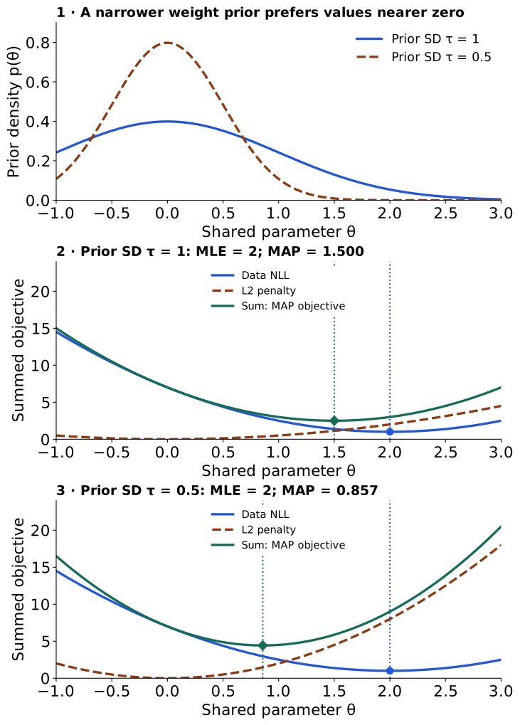
This prior acts on a shared parameter; \(\tau^2\) is distinct from observation-noise variance \(\sigma^2\). MAP retains one setting, not posterior spread, and a mode need not equal a posterior mean.
Reduction changes the coefficient. Dividing the entire MAP objective by \(n\), or rescaling it using the fixed-variance Gaussian relation in Common variance gives scaled squared error, preserves its optimizer:
| Data-loss convention | Penalty giving the same MAP fit |
|---|---|
| Summed NLL \(\sum_i L_i\) | \(\|\theta\|_2^2/(2\tau^2)\) |
| Mean NLL \(\bar L\) | \(\|\theta\|_2^2/(2n\tau^2)\) |
| MSE without a factor \(1/2\) | \(\sigma^2\|\theta\|_2^2/(n\tau^2)\) |
The MSE row assumes fixed common \(\sigma^2\). BCE and CE can receive the same prior penalty using their NLL convention. Declare which parameters have this prior, including whether biases are penalized.
This CPU example includes both intercept and slope in \(\theta=(b,w)\) and uses unit observation variance. The omitted Gaussian normalization is constant in these weights:
import torch

x = torch.tensor([[-1.0], [0.0], [1.0]])
y = torch.tensor([[1.0], [2.0], [3.0]])
theta = torch.tensor([0.2, 0.4], requires_grad=True)  # b, w
prediction = theta[0] + theta[1] * x               # (B, 1)
n_train, tau = len(y), 0.5
mean_nll = 0.5 * (y - prediction).square().mean()
l2 = theta.square().sum() / (2 * n_train * tau**2)
loss = mean_nll + l2
loss.backward()
assert torch.isfinite(loss) and torch.isfinite(theta.grad).all()
For minibatch estimates of this mean objective, n_train remains the full training-set size, not batch size \(B\). This explicit loss penalty is not generally equivalent to decoupled AdamW weight decay (Loshchilov and Hutter 2019). Next we will compare a point estimate with keeping and predicting from a posterior.
An exact binary-probability update
Return to the separate ten-event sequence in Maximum likelihood and negative log likelihood: three rain events and seven dry events. Here \(\mathcal D\) denotes these ten outcomes. Assume independent Bernoulli outcomes with one constant, unknown rain rate \(\rho\). This is a synthetic model, not a claim that real weather is independent across days.
Put a Beta prior on the unknown probability. Its positive shape parameters \(\alpha\) and \(\beta\) determine a density on \(0<\rho<1\):
\[ p(\rho)\propto\rho^{\alpha-1}(1-\rho)^{\beta-1}. \]
Choose \(\alpha=2\), \(\beta=3\), giving prior mean \(2/(2+3)=0.4\). Multiplying by the ordered-sequence likelihood gives
\[ \begin{aligned} p(\rho\mid\mathcal D) &\propto\underbrace{\rho^3(1-\rho)^7}_{\text{likelihood}} \underbrace{\rho^{2-1}(1-\rho)^{3-1}}_{\text{prior}}\\ &=\rho^{5-1}(1-\rho)^{10-1}. \end{aligned} \]
This is the kernel of \(\operatorname{Beta}(5,10)\); normalization identifies the full posterior. We chose a prior family that stays in the same family after updating—a conjugate prior (Bishop 2006, sec. 2.1.1). Compare three summaries:
| Summary | Value | What it retains |
|---|---|---|
| MLE | \(3/10=0.3\) | Maximum of the likelihood |
| Interior posterior mode, MAP | \((5-1)/(5+10-2)=4/13\) | Maximum of the posterior density |
| Posterior mean | \(5/(5+10)=1/3\) | Average under the posterior |
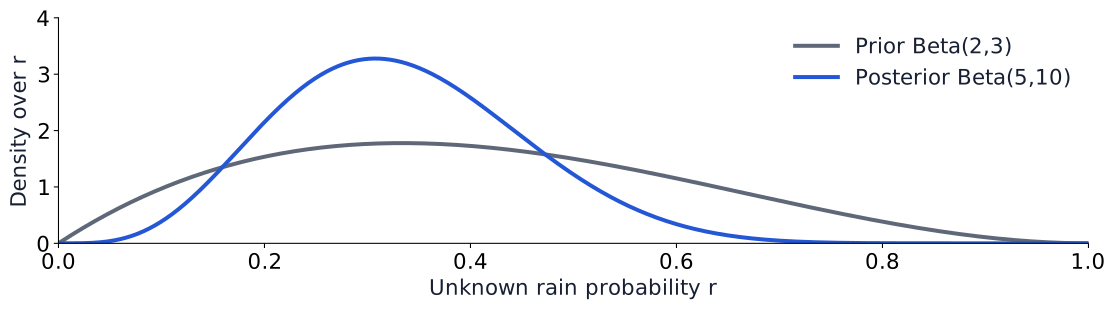
Keeping the full curve in Figure 7 lets prediction average over plausible rates. Write \(Y_*\) for the outcome of one new Bernoulli event. The subscript \(*\) means new or future, rather than one of the training observations; it is a label, not multiplication. This convention will also apply to \(x_*\), \(y_*\) and other quantities at a new input. Then
\[ \begin{aligned} P(Y_*=1\mid\mathcal D) &=\int_0^1\rho\,p(\rho\mid\mathcal D)\,d\rho\\ &=\mathbb E[\rho\mid\mathcal D]=\frac13. \end{aligned} \]
The mean arises from this predictive integral, not from selecting the most probable parameter. A posterior density over a probability and a predictive probability of rain answer different questions.
Bayesian regression: uncertain weights and future readings
A line has two unknowns rather than one rain rate. Use the tutorial’s \(n=20\) synthetic observations, known noise SD \(\sigma=0.25\), and prior SD \(\tau=1.5\). Let \(\theta=(b,w)^\top\) contain intercept \(b\) and slope \(w\); the superscript \(\top\) transposes a row into a column (and vice versa). For this calculation, form a design matrix \(X\) whose rows are \([1,x_i]\): \(X\) has shape \((n,2)\), \(\theta\) has shape \((2,1)\), and the target column \(\mathbf y\) has shape \((n,1)\). The notebook represents vectors as one-dimensional NumPy arrays.
Write \(I_k\) for the \(k\times k\) identity matrix, with ones on its diagonal and zeros elsewhere. Assume
\[ \theta\sim\mathcal N(0,\tau^2I_2),\qquad \mathbf y\mid X,\theta\sim\mathcal N(X\theta,\sigma^2I_n). \]
Both intercept and slope receive the prior. Multiplication gives a posterior proportional to
\[ \exp\!\left[-\frac12\left( \frac{\|\mathbf y-X\theta\|_2^2}{\sigma^2} +\frac{\theta^\top\theta}{\tau^2}\right)\right]. \]
Expand the squared residual:
\[ \begin{aligned} \|\mathbf y-X\theta\|_2^2 &=\mathbf y^\top\mathbf y-2\theta^\top X^\top\mathbf y\\ &\quad+\theta^\top X^\top X\theta. \end{aligned} \]
After collecting terms, define the \((2,2)\) precision matrix \(A\) and the \((2,1)\) column \(m\) by the following linear system. A negative scalar power denotes a reciprocal, for example \(\sigma^{-2}=1/\sigma^2\):
\[ A=\tau^{-2}I_2+\sigma^{-2}X^\top X, \qquad Am=\sigma^{-2}X^\top\mathbf y. \]
Completing the square turns the parameter-dependent expression into
\[ \begin{aligned} \theta^\top A\theta-2\theta^\top Am &=(\theta-m)^\top A(\theta-m)-m^\top Am. \end{aligned} \]
The final term is constant in \(\theta\). Write \(S_\theta=A^{-1}\) for the posterior covariance; \(A^{-1}\) denotes the matrix inverse. Here \(\mathcal N(\theta;m,S_\theta)\) means a Gaussian density evaluated at \(\theta\), with mean \(m\) and covariance \(S_\theta\). Recognizing the normalized Gaussian gives
\[ \begin{aligned} p(\theta\mid\mathcal D)&=\mathcal N(\theta;m,S_\theta),\\ S_\theta&=A^{-1},\qquad m=S_\theta\sigma^{-2}X^\top\mathbf y. \end{aligned} \]
\(S_\theta\) is the posterior covariance: its diagonal entries describe uncertainty in intercept and slope; its off-diagonal entries describe how their uncertainties vary together. Precision is inverse covariance. Prior and data precision add in this model. The proper Gaussian prior makes \(A\) positive definite. This posterior’s mean equals its mode, so \(m\) also gives the ridge/MAP fit. Keeping only \(m\) discards \(S_\theta\) (Bishop 2006, sec. 3.3).
At a new input \(x_*\), let \(y_*\) be a future noisy target. Define the row vector \(a_*=[1,x_*]\) and mean function \(f_*=a_*\theta\). Then
\[ \mathbb E[y_*\mid x_*,\mathcal D]=a_*m, \]
\[ \operatorname{Var}(y_*\mid x_*,\mathcal D) =\underbrace{a_*S_\theta a_*^\top}_{\text{uncertainty in the mean}} +\underbrace{\sigma^2}_{\text{observation noise}}. \]
This is the law of total variance: average the conditional noise variance, then add the variance of the conditional mean. One posterior weight draw specifies an entire plausible line; a future noisy reading adds another source of variation.
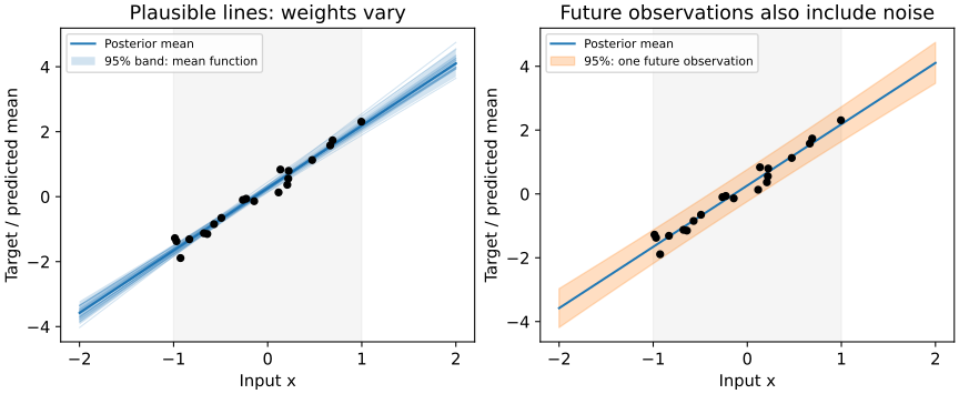
Figure 8 separates the two uncertainties. Its intervals are not simultaneous bands for an entire curve or guarantees under distribution shift. The tutorial’s regression calculation uses linear solves for the displayed equations. The exact Gaussian answer relies on a mean linear in the weights, Gaussian noise and a Gaussian prior; a nonlinear neural network generally loses this closed form.
From exact inference to approximate neural-network prediction
The examples above permit normalized posteriors and predictive calculations. What becomes difficult when the same probability argument uses a large neural network?
Why exact Bayesian inference becomes difficult
Many weights interact through nonlinear layers, so the likelihood times prior rarely simplifies to a familiar normalized density. Plausible settings may form correlated regions or separated modes. Evidence integrates over all of them; prediction requires another weighted average:
\[ \begin{aligned} p(y_*\mid x_*,\mathcal D) =\int &p(y_*\mid x_*,\theta)\\ &\times p(\theta\mid\mathcal D)\,d\theta. \end{aligned} \]
The obstacle is not continuity alone: the preceding continuous regression model was tractable. It is the combination of dimension, posterior shape and repeated integration.
Markov chain Monte Carlo constructs dependent samples targeting a posterior; it can use an unnormalized density, although exploring that density well may be expensive. Variational inference instead fits a tractable approximating distribution. An unavailable normalizer therefore does not make all Bayesian computation impossible. These methods introduce computational or approximation tradeoffs, and neither fixes a poorly specified observation model automatically (Bishop 2006, sec. 10.1).
Monte Carlo dropout: prediction with sampled masks
Let \(T\) be the number of stochastic passes. Superscripts \((t)\) label draws, \(t=1,\ldots,T\), rather than powers. Suppose we can draw approximate weight settings \(\theta^{(1)},\ldots,\theta^{(T)}\). The predictive integral becomes a Monte Carlo average of the corresponding observation distributions. Yarin Gal and Zoubin Ghahramani showed how dropout training and stochastic prediction admit an approximate Bayesian interpretation (Gal and Ghahramani 2016, secs. 3–4). Under their construction, dropout masks define a restricted distribution over effective network weights; its training objective links the data fit and regularization to variational inference.
This gives a practical bridge: train with dropout, then keep those dropout layers active for repeated prediction. It does not justify inserting dropout into an arbitrary finished network. The tutorial illustrates the stochastic prediction mechanism; it does not reproduce a fully matched paper-level prior and regularization specification or demonstrate calibrated posterior probabilities.
For scalar regression, masked mean predictions \(\widehat y_*^{(t)}\) give empirical mean \(\bar y_*\) and mask variance \(v_{\mathrm{masks}}\):
\[ \bar y_*=\frac1T\sum_t\widehat y_*^{(t)},\qquad v_{\mathrm{masks}}=\frac1T\sum_t(\widehat y_*^{(t)}-\bar y_*)^2. \]
This empirical spread omits observation noise. Add the average conditional noise variance for a full predictive-variance approximation. For classification, average the probabilities from each pass, rather than averaging logits before applying sigmoid or Softmax.
This function matches the tutorial’s registered torch.nn.Dropout modules and real-valued mean output. Other layers remain in evaluation mode (PyTorch contributors, n.d.-c):
import torch

def dropout_predictions(model, x, passes=100):
    assert passes > 1
    model.eval()
    try:
        for layer in model.modules():
            if isinstance(layer, torch.nn.Dropout):
                layer.train()
        with torch.no_grad():
            draws = torch.stack([model(x) for _ in range(passes)])
    finally:
        model.eval()
    return draws.mean(0), draws.var(0, unbiased=False)
For input shape \((B,1)\) and scalar output \((B,1)\), the stacked predictions have shape \((T,B,1)\); both returned arrays have shape \((B,1)\). The variance uses the empirical \(1/T\) convention above. Evaluation mode is restored even if prediction fails.
Read the tutorial dropout scene with two limitations in mind. Independent masks per batch row mean a plotted pass need not be one coherent posterior function draw across all inputs. Also, its nonlinear MLP and the exact straight-line model belong to different function families; their plots cannot rank inference methods. Mask spread does not guarantee widening uncertainty outside the training range, calibration, or robustness.
A VAE performs approximate Bayesian inference over latent codes
So far the uncertain quantities were a rain rate or shared regression weights. A variational autoencoder (VAE) introduces an unobserved code for each image. Its Bayesian inference concerns that code; the ordinary VAE here still learns point estimates of its network weights (Kingma and Welling 2014).
Generate an image forward; infer its code backward
Notation changes at this boundary: \(x\) now denotes a whole observed image, not a scalar regression input. Write \(u\in\mathbb R^d\) for its latent code: \(\mathbb R^d\) is the space of real vectors with \(d\) coordinates, and \(d\) now denotes latent dimension. Write \(\theta\) for decoder weights, and \(\psi\) for encoder weights. Kingma and Welling use \(z\) and \(\phi\) for our \(u\) and \(\psi\); we reserve \(\phi\) for the course’s activation function.
A generative model tells a forward story (\(I_d\) is the \(d\times d\) identity matrix):
\[ \begin{aligned} u&\sim p(u)=\mathcal N(0,I_d),\\ x\mid u,\theta&\sim p(x\mid u,\theta),\\ p(x,u\mid \theta)&=p(x\mid u,\theta)p(u). \end{aligned} \]
The decoder supplies the parameters of an image observation distribution. Given an image, inference asks the reverse question: which codes could have generated it? Bayes’ rule gives
\[ \begin{aligned} p(u\mid x,\theta)&=\frac{p(x\mid u,\theta)p(u)}{p(x\mid \theta)},\\ p(x\mid \theta)&=\int p(x\mid u,\theta)p(u)\,du. \end{aligned} \]
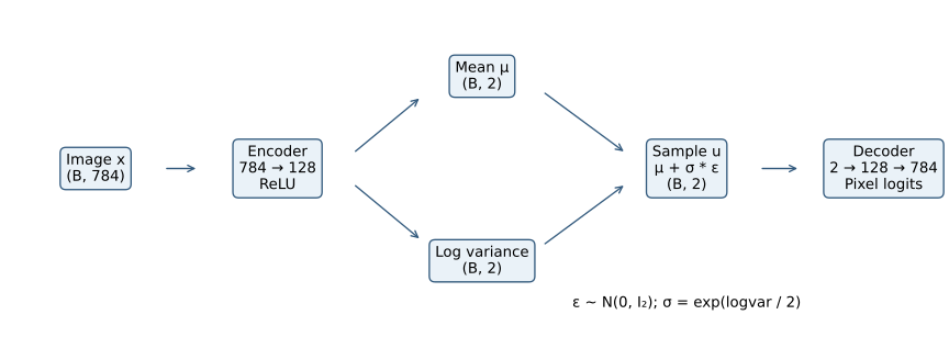
The nonlinear decoder generally makes this integral and posterior intractable. An encoder instead outputs a mean vector \(\mu_u(x)\) and log-variance vector \(\ell_u(x)\) for a tractable approximation. The operator \(\operatorname{diag}\) places a vector on a matrix’s diagonal; exponentiation acts on each coordinate:
\[ q(u\mid x,\psi)=\mathcal N\!\left( u;\mu_u(x),\operatorname{diag}(\exp(\ell_u(x)))\right). \]
Here \(\ell_u\) is a vector of log variances, not log standard deviations. A Gaussian approximation does not imply that the exact posterior is Gaussian. One shared encoder maps many images to their own distributions; this reuse is called amortized inference.
| Model | Observed | Unknown being inferred | Retained distribution |
|---|---|---|---|
| Bayesian regression | Training pairs | Shared weights \(\theta\) | \(p(\theta\mid\mathcal D)\) |
| This VAE | An image \(x\) | Its code \(u\) | Approximation \(q(u\mid x,\psi)\) |
The prior, observation model, and posterior target make this Bayesian inference. Randomness in a bottleneck alone would not establish that interpretation. No posterior over \(\theta\) or \(\psi\) is retained here.
From Bayes’ rule to the evidence lower bound
How should we train the approximation and decoder? Here \(q\) and \(p\) stand for the two densities being compared, and \(\mathbb E_q\) means averaging over draws from \(q\). Define the Kullback–Leibler divergence (KL) between two densities on the same space:
\[ D_{\mathrm{KL}}(q\|p)=\mathbb E_q[\ln q(u)-\ln p(u)]\geq0. \]
It measures a directed discrepancy, not a symmetric distance. We assume the integrals below are finite and \(p\) is positive wherever \(q\) places mass. Start with the discrepancy to the posterior, and substitute Bayes’ rule:
\[ \begin{aligned} &D_{\mathrm{KL}}(q(u\mid x,\psi)\|p(u\mid x,\theta))\\ &\quad=\mathbb E_q[\ln q(u\mid x,\psi)-\ln p(u\mid x,\theta)]\\ &=\mathbb E_q[\ln q(u\mid x,\psi)-\ln p(u)\\ &\qquad-\ln p(x\mid u,\theta)+\ln p(x\mid \theta)]. \end{aligned} \]
The image evidence \(p(x\mid \theta)\) is constant with respect to \(u\), so its log leaves the expectation. Rearranging gives the key identity:
\[ \begin{aligned} \ln p(x\mid \theta) &=\mathcal E(\theta,\psi;x)\\ &\quad+D_{\mathrm{KL}}(q(u\mid x,\psi)\|p(u\mid x,\theta)),\\[2pt] \mathcal E(\theta,\psi;x) &=\underbrace{\mathbb E_q[\ln p(x\mid u,\theta)]}_{\text{expected reconstruction log likelihood}}\\ &\quad-\underbrace{D_{\mathrm{KL}}(q(u\mid x,\psi)\|p(u))}_{\text{discrepancy to the prior}}. \end{aligned} \]
Nonnegative posterior divergence makes \(\mathcal E\) an evidence lower bound (ELBO). We can optimize it without evaluating the evidence integral (Kingma and Welling 2014, sec. 2.2). Notice the two different divergences: the posterior KL is the gap to log evidence; the prior KL is a computable term inside the bound. Even if \(q\) equals the posterior, the prior KL need not vanish.
With the decoder fixed, improving \(q\) tightens this bound toward fixed evidence. Joint training also changes \(\theta\), so the evidence itself changes. It cannot be discarded as constant when optimizing decoder weights. Finally, the bound concerns the exact expectation: one Monte Carlo reconstruction estimate can lie above log evidence without contradicting the identity.
Reparameterization connects the bound to trainable networks
To differentiate through a code sample, draw independent standard Gaussian noise \(\epsilon\) for each image and write the sample as:
\[ \epsilon\sim\mathcal N(0,I_d),\qquad u=\mu_u(x)+\exp(\ell_u(x)/2)\odot\epsilon. \]
\(\odot\) means elementwise multiplication. Holding the sampled \(\epsilon\) fixed during a backward pass makes \(u\) a differentiable function of both encoder heads. New forward passes draw new noise. Gradients reach the mean head, log-variance head, and decoder; the factor \(1/2\) converts log variance to log standard deviation.
Below, \(j\) indexes pixels and \(k\) indexes latent coordinates. The tutorial thresholds MNIST pixels to \(x_j\in\{0,1\}\). Its decoder outputs 784 logits, defining conditionally independent Bernoulli pixels with probabilities \(\widehat x_j(u)\). The independence assumption is given the code; sharing a random code can still make pixels dependent marginally. As in Bernoulli: from two cases to binary cross-entropy, taking the negative log likelihood gives
\[ \begin{aligned} -\ln p(x\mid u,\theta) =-\sum_{j=1}^{784}\big[&x_j\ln\widehat x_j(u)\\ &+(1-x_j)\ln(1-\widehat x_j(u))\big]. \end{aligned} \]
This is summed pixel BCE, not an arbitrary image-distance choice. For the diagonal Gaussian encoder and standard normal prior, the other term has a closed form:
\[ D_{\mathrm{KL}}(q(u\mid x,\psi)\|p(u)) =\frac12\sum_{k=1}^d\left[ \mu_{u,k}^2+\exp(\ell_{u,k})-1-\ell_{u,k}\right]. \]
Minimizing negative ELBO therefore means expected reconstruction BCE plus this prior KL. The tutorial estimates the expectation with one sampled code per image, sums over pixels and code coordinates, then averages over batch images. Both terms have coefficient one. Averaging BCE over pixels while leaving KL unchanged would alter their relative weight and the objective.
For batch size \(B\), image/logit shapes are \((B,784)\); mean and log variance are \((B,2)\) in the two-dimensional example. Each summed term has shape \((B,)\) before the final batch mean. The tutorial’s two-term loss and gradient checks implement this calculation with stable BCE on logits.
For reconstruction, decoding the encoder’s mean code is a useful display, but generally differs from averaging decoded outputs. For generation, draw a fresh code from the prior and decode its pixel probabilities; optionally sample binary pixels from them. A small reconstruction error alone does not establish good prior samples or interpretable latent coordinates.
Frequentist and Bayesian approaches: what changes?
Both approaches need a defensible observation model. BCE, categorical CE, and Gaussian regression NLL came from that model before any prior was introduced. The distinction is how unknown quantities and uncertainty are handled. The table compares the specific fitting methods developed here, not every method in either tradition.
| Question | Frequentist MLE | MAP | Retained Bayesian posterior |
|---|---|---|---|
| How are weights treated? | Fixed unknown parameters | Search for one posterior mode | Represent uncertainty by a distribution |
| What determines the fit? | Likelihood | Likelihood and prior | Likelihood and prior |
| What is retained? | One maximizing setting | One maximizing setting | Exact or approximate posterior |
| How is a new outcome predicted? | Observation model at fitted weights | Observation model at MAP weights | Average observation models over the posterior |
| What uncertainty is available directly? | Observation-model variability | Observation-model variability | Observation noise and parameter uncertainty |
| What computation is needed here? | Optimization | Penalized optimization | Integration, sampling, or approximation |
Frequentist analysis also quantifies estimation uncertainty, for example through confidence intervals or bootstrap resampling. It is not restricted to point predictions. A frequentist 95% confidence procedure covers the fixed true parameter in 95% of repeated datasets under its assumptions. A 95% Bayesian credible region contains 95% posterior probability conditional on the observed data, model, and prior. Neither interpretation guarantees reliability after distribution shift or model misspecification (Bishop 2006, sec. 1.2.3).
MAP connects the two computational workflows: a Gaussian weight prior produces the familiar L2-regularized loss, with the coefficient determined by the loss reduction. Nevertheless, a single MAP setting cannot supply the predictive integral or posterior covariance. Conversely, an approximate distribution is useful only to the extent that its assumptions and approximation are adequate.
Ask three questions when reading a learning objective: What is observed? What is unknown? What is retained? In binary classification, the network specifies a distribution over labels. Bayesian regression also retains uncertainty over shared weights. Dropout supplies a restricted approximate inference mechanism. The VAE infers a distribution over each image’s hidden code while fitting point-valued network weights. These distinctions explain both where the losses come from and what their trained outputs can tell us.
Questions and exercises (optional)
These questions revisit the derivations; they do not require VAE training.
Read a conditional carefully. Using Table 1, calculate \(P(R=1\mid S=0)\) and \(P(S=0\mid R=1)\). State each denominator in words. Why do the answers describe different sensor questions?
Derive the selectors. Check the Bernoulli expression \(\widehat y^{\,y}(1-\widehat y)^{1-y}\) for both labels. Extend the argument to a three-class one-hot target and derive mean dataset NLL. State the independence assumption used between observations.
Learn a variance responsibly. Hold a nonzero regression residual fixed. What happens if a model minimizes only its squared residual divided by predicted variance? Explain the role of the log-variance term in Gaussian NLL. Why is the density at one exact target not the probability of that target?
Keep the prior scaling. Start with summed NLL plus \(\|\theta\|^2/(2\tau^2)\) for \(n\) training examples. Rewrite the same objective with mean NLL. For a uniform minibatch of size \(B\), give an unbiased estimate of that mean objective and identify where \(n\) and \(B\) appear.
Separate two intervals. In the linear-Gaussian example, write the variance of the uncertain mean at \(x_*\) and the variance of a future reading there. Explain what is added, why, and which interval would remain wider if parameter uncertainty became very small.
Locate the Bayesian inference. For the VAE, name the observed variable, latent unknown, fitted weights, and approximate posterior. In the ELBO identity, which KL is the gap and which is part of the training objective? If the encoder matched the exact posterior, would both KL terms be zero? Justify from their arguments.