← Course homeAll chapters

Week 10 · Discovering Structure with Unsupervised Learning

NoteDraft for instructor review

The introduction and PCA explanation have been reviewed. The chapter now includes t-SNE, clustering, autoencoders and variational autoencoders. TODO(instructor): review the remaining method sections, figures, and the revised explanatory sequence before accepting the complete chapter.

Imagine a collection of handwritten digits with their names removed. Each image still contains measurements: the intensity of every pixel. Some images resemble one another; some share a stroke but differ elsewhere. We can ask whether a few numbers could describe these differences, whether the images form useful groups, or whether a model could produce new examples.

Those are different questions about the same observations. To answer one, we must decide what structure to preserve and how to recognize success. This chapter develops that decision through geometry, representations, and eventually models of how observations could arise.

Planned learning outcomes. As the chapter is developed, you will learn to:

• distinguish compression, clustering, visualization, and generation by their objectives and evidence;
• derive PCA from projection and reconstruction, and explain what it preserves;
• trace how t-SNE constructs a neighborhood map and interpret its limitations;
• explain how a clustering objective determines assignments and centers; and
• connect learned representations to reconstruction and latent generative models.

Prerequisites and companions. We assume vectors, matrix multiplication, and basic derivatives. The Week 04 chapter introduces learned representations and the training loop; Week 07 develops probability, likelihood, and latent-variable inference. We will recall the needed geometry and probability at the point of use. The current Week 10 lecture and tutorial are earlier drafts awaiting revision to follow this chapter.

Reading route. PCA compresses observations with a linear projection; t-SNE builds a map of local relationships. K-means and Gaussian mixtures turn a chosen notion of resemblance into group membership. Autoencoders learn nonlinear codes for reconstruction. Variational autoencoders add a probability model that supplies new codes and generates observations. The final section returns to the four questions below and checks what each experiment has established.

Learning from observations without supplied answers

In supervised learning, each training observation comes with a target for a specified task: an image and its digit label, for example. Unsupervised learning fits structure from observations without using such task labels as fitting targets. A dataset can have labels stored elsewhere and still support an unsupervised experiment: the relevant question is what information enters fitting (Goodfellow et al. 2016, chap. 5).

Write the observations as \(\mathcal D=\{x_i\}_{i=1}^n\), where \(x_i\) contains \(D\) measurements. A representation is a description of an observation in coordinates chosen for a purpose. For an image, those coordinates might describe combinations of pixels rather than individual pixel intensities. An encoder maps an observation to its representation, \(h_i=f_\theta(x_i)\). Reducing the number of coordinates is one possible purpose; an encoder does not have to reduce dimension.

What makes one representation better than another? The answer depends on the question. If we want to store images economically, retaining enough information to reconstruct them matters. If we want to explore which images resemble one another, preserving local relationships may matter more. The absence of supplied labels leaves us responsible for specifying a learning objective: the quantity that fitting tries to improve. It also leaves choices about measurements, scaling, model family, and evaluation.

Four questions, four kinds of evidence

The same collection of images can support all four investigations below. Each row pairs a question with evidence that addresses it.

Ask the model to…	Question about the result	Evidence to examine
Compress	Can fewer coordinates retain enough information to recover an observation?	Reconstruction error; use held-out observations when claiming performance on new data.
Group	Does a chosen notion of similarity produce useful groups?	Compactness under that metric, stability under stated perturbations, and external diagnostics when available.
Map	Does a low-dimensional picture preserve relationships we want to inspect?	Neighborhood preservation and sensitivity to mapping choices.
Generate	Does the fitted model produce observations consistent with the intended distribution?	Samples from its specified sampling procedure and model diagnostics; attractive examples alone are insufficient.

Suppose two images fall close together on a map. That is a statement about the map’s coordinates. Whether they belong to the same digit class is a separate question. Similarly, reconstructing a stroke accurately does not establish that a representation makes its digit name easy to predict. We can investigate that usefulness with a declared downstream task, such as fitting a classifier to fixed representations. Labels used for that classifier must be distinguished from information used to fit the representation.

The table is therefore a guide to choosing an experiment. We will first understand what a method computes, then ask what evidence its result supports.

Why this matters for modern machine learning

Learning from observations without separately supplied task labels connects this chapter to self-supervised learning (SSL). In a self-supervised task, the observations themselves supply the prediction targets or relationships used in training. For example, in next-token language-model pretraining, a text prefix is the input and the following token supplies a target. The text already contains the training pairs; a person need not attach a separate answer to each prefix. Autoregressive pretraining in GPT-3 is a concrete example (Brown et al. 2020).

Another example learns image representations by comparing transformed views of the same image with views of other images. SimCLR shows how a contrastive objective can support this form of representation learning (Chen et al. 2020). These examples make a distinction useful throughout this chapter: where training information comes from and what the objective rewards are related but separate questions. We use “self-supervised” when targets or comparison relationships are constructed from the observations, and “unsupervised” for the broader setting without supplied task labels as fitting targets.

This is the connection that matters for our 2026 course: projection, reconstruction, and neighborhood objectives give us manageable settings in which to examine what a learning rule retains. The same question can then be asked of a large language model (LLM). This does not make PCA a model of language-model training; it gives us a precise way to discuss a representation and its purpose.

Reinforcement learning (RL) adds decisions and rewards. An agent may use a learned representation of its observations, but its decision objective concerns reward. We will keep that distinction when connecting representation learning to later course material.

Abbreviations and notation reference

Use this reference when a symbol or abbreviation is unfamiliar. Each method introduces its quantities where they are needed; there is no need to memorize the tables before reading.

Abbreviation	Meaning
PCA; SVD	Principal component analysis; singular value decomposition
t-SNE	t-distributed stochastic neighbor embedding
AE; VAE	Autoencoder; variational autoencoder
GMM; EM	Gaussian mixture model; expectation–maximization
MSE	Mean squared error
NLL; BCE	Negative log likelihood; binary cross-entropy
KL; ELBO	Kullback–Leibler divergence; evidence lower bound
SSL; LLM; RL	Self-supervised learning; large language model; reinforcement learning
UMAP	Uniform manifold approximation and projection; optional comparison

SSL means self-supervised, rather than semi-supervised, learning here. A cluster is a group produced under a specified criterion; a class is a task category. An embedding is a coordinate representation; a latent variable is an unobserved variable in a model. We will distinguish these roles rather than infer one from a picture.

Symbols	Meaning and shape convention
\(n,D,d\)	Number of observations, input dimension, representation dimension
\(x_i\), \(X\in\mathbb R^{n\times D}\)	Observation as a column vector; data matrix with row \(i\) equal to \(x_i^\top\)
\(\bar x\), \(X_c\)	Training mean vector and data centered using that mean
\(h_i\), \(H\in\mathbb R^{n\times d}\)	Representation vector and matrix of representations as rows
\(\widehat x_i\); \(y_i\)	Reconstructed observation; an external task label, when available
\(V\in\mathbb R^{D\times d}\)	PCA basis with orthonormal columns; \(H=X_cV\)
\(K\), \(a_i\), \(c_k\), \(n_k\)	Cluster count, assignment of observation \(i\), center of cluster \(k\), and its membership count
\(v_i\in\mathbb R^2\); \(P_{ij},Q_{ij}\); \(\tau_i\)	t-SNE map coordinate; input/map joint affinities; input bandwidth
\(\theta\), \(L_i\), \(L\)	Model parameters, per-observation loss, and objective with its reduction stated locally
\(\mathbf{z}\), \(p_\theta(\mathbf{x}\mid \mathbf{z})\), \(q_\psi(\mathbf{z}\mid \mathbf{x})\)	Stochastic latent variable, decoder observation model, and encoder approximate posterior

A transpose is denoted by \(\top\); a hat marks a reconstruction or estimate and a bar an average. Indices \(i,j\) refer to observations unless explicitly stated otherwise; \(k\) indexes clusters. We retain \(W^{(\ell)}\), \(b^{(\ell)}\), \(z^{(\ell)}\), \(h^{(\ell)}\), and \(\phi\) for layer weights, biases, preactivations, representations, and activation functions from Week 04. In a VAE, \(\theta\) will refer specifically to decoder parameters and \(\psi\) to encoder parameters. Specialized distribution parameters, tensor shapes, and sums or averages will be defined before their calculations.

Dimensionality reduction: PCA and t-SNE

A photograph may contain millions of pixel measurements, but nearby pixels often vary together. Keeping every coordinate can repeat information. A smaller representation can reduce storage and the cost of later computations; two or three coordinates can also give us a view of a dataset. These purposes need not favor the same representation. Two coordinates useful for a picture may discard information needed for reconstruction or prediction.

An encoder gives us a useful language for this task: map an observation \(x_i\in\mathbb R^D\) to coordinates \(h_i\in\mathbb R^d\). For dimension reduction, \(d<D\). If reconstruction matters, add a decoder that maps those coordinates back to an approximation \(\widehat x_i\). We will begin with a linear encoder and decoder, where every operation can be drawn. PCA chooses their directions using the data (Goodfellow et al. 2016, chap. 13).

PCA: projection, variation, and reconstruction

How can we replace many measurements with fewer coordinates while retaining enough information to recover the observations? Principal component analysis (PCA) answers this question within a linear model: it chooses orthogonal directions that retain as much squared variation as possible. The same choice minimizes squared reconstruction error. We will first build a visual intuition and recall covariance, then state the two algorithms. The derivation will explain why they work; one complete numerical example will show how to use them. Finally, we will examine image representations and the limits of linear projection.

One coordinate is a position along a line

Imagine measuring two features of each object. An observation is a point in a plane. Keeping only the first feature projects it onto the horizontal axis; keeping only the second projects it onto the vertical axis. We can also choose an oblique line and record each point’s position along it. The line is shared by all observations; each observation gets its own coordinate.

Encoding records that coordinate. Reconstruction places the observation back on the line at the recorded position. Any displacement perpendicular to the line has been discarded. PCA’s task is to choose a line—or, with more retained coordinates, a subspace—that keeps as much variation as possible. We will state the procedure before deriving the criterion that selects it.

Figure 1: The same cloud can be described along different directions. A single retained coordinate should follow a direction that preserves useful variation.

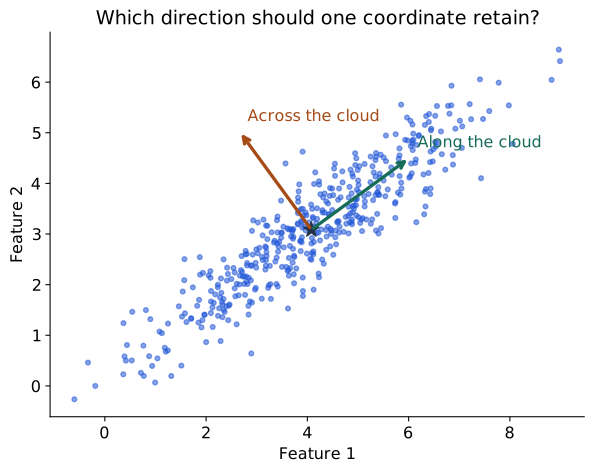
The star marks the average observation. The arrows suggest two perpendicular directions: along the cloud and across it. A signed position along an arrow is a coordinate. Keeping one such position compresses each observation to one number. The algorithms below will specify how to choose and use that direction; we will then revisit the full change of coordinates.

Recap: covariance measures joint variation

Variance describes how one measurement varies around its mean. Covariance asks whether two measurements tend to deviate from their respective means together. Imagine each observation has a height and a weight. For each person, subtract the mean height and the mean weight, then multiply the two deviations. A person above both means gives a positive product; someone below both means also gives a positive product. Being above one mean and below the other gives a negative product. Covariance averages these signed contributions.

For scalar random variables \(A,B\) with finite second moments, the population definition is

\[ \operatorname{Cov}(A,B)= \mathbb E[(A-\mathbb E[A])(B-\mathbb E[B])]. \]

Expanding the product and using linearity of expectation gives \(\mathbb E[AB]-\mathbb E[A]\mathbb E[B]\). Setting \(B=A\) recovers variance: \(\operatorname{Cov}(A,A)=\operatorname{Var}(A)\). Swapping the variables leaves the product unchanged, so covariance is symmetric (Bishop 2006, sec. 1.2.2).

In a dataset, replace the expectation by an average over paired observations. Each pair must come from the same observation; multiplying unrelated heights and weights would lose the relationship being measured. The following small examples use equally weighted observations and denominator \(n=3\):

First feature values	Second feature values	Covariance	Interpretation
\((-1,0,1)\)	\((-2,0,2)\)	\(4/3\)	Deviations have matching signs.
\((-1,0,1)\)	\((2,0,-2)\)	\(-4/3\)	Deviations have opposing signs.
\((-1,0,1)\)	\((1,0,1)\)	\(0\)	Positive and negative products cancel, even though the second feature is the square of the first.

For the last row, the second feature’s mean is \(2/3\). The centered products are \(-1/3,0,1/3\), whose average is zero. Zero covariance does not establish independence: a nonlinear relationship can remain. A constant feature also has zero covariance with every feature.

Covariance has the product of the two measurement units. Changing a measurement’s scale changes the number, so covariance magnitudes from different units cannot be read as a universal measure of association strength. For positive variances, correlation removes those units:

\[ \rho_{AB}=\frac{\operatorname{Cov}(A,B)} {\sqrt{\operatorname{Var}(A)\operatorname{Var}(B)}}. \]

Correlation is undefined when either variance is zero. PCA on centered original features uses covariance; PCA after standardizing each nonconstant feature uses its correlation matrix, under matching variance conventions. Choosing between them determines which feature scales the method treats as important.

Scaling a feature changes squared distances and covariance. Converting metres to centimetres multiplies that feature’s deviations by 100 and its variance by 10,000. If this change of units should not dominate the representation, standardizing features using training means and standard deviations may be appropriate. If absolute magnitudes carry the scientific meaning, standardizing can remove something valuable. Centering and scaling are distinct operations; a constant feature requires explicit handling before division by its standard deviation.

With many features, put all pairwise covariances into one matrix. Its diagonal contains feature variances; its symmetric off-diagonal entries describe joint variation. This matrix will let us calculate the variance along any proposed projection direction.

Reading the procedure: data, directions, and scores

Let \(X\in\mathbb R^{n\times D}\) contain observations as rows. Write \(x_i\) for one observation as a column vector, \(\bar x\) for the training mean, and \(\widetilde x_i=x_i-\bar x\) for its centered version. The centered matrix \(X_c\) has rows \(\widetilde x_i^\top\). With our \(1/n\) convention, the covariance matrix is

\[ C=\frac1n X_c^\top X_c\in\mathbb R^{D\times D},\qquad C_{ab}=\frac1n\sum_i\widetilde x_{i,a}\widetilde x_{i,b}. \]

Here \(a,b\) index features. Each observation contributes all pairwise deviation products through the \(D\times D\) outer product \(\widetilde x_i\widetilde x_i^\top\). Averaging these matrices gives \(C\).

An eigenvector \(v_j\) of \(C\) satisfies \(Cv_j=\lambda_jv_j\): the matrix scales it by \(\lambda_j\) without changing its line. A symmetric covariance matrix supplies mutually perpendicular unit directions. PCA keeps those with the largest eigenvalues. We will derive why eigenvalues measure retained variance immediately after the algorithms.

Put the retained directions in the columns of \(V\in\mathbb R^{D\times d}\). Then \(V^\top V=I_d\), where \(I_d\) is the identity matrix. The vector \(\mathbf1_n\) contains \(n\) ones; multiplying it by \(\bar x^\top\) repeats the mean across all rows. These conventions let us state the complete encoding and reconstruction procedures now.

Algorithm 1: fit PCA and reduce the feature space

Input: training matrix \(X\in\mathbb R^{n\times D}\) with observations in rows and a retained dimension \(1\le d\le D\). Assume finite numeric measurements and \(n\ge2\). Output: fitted mean \(\bar x\in\mathbb R^D\), basis \(V\in\mathbb R^{D\times d}\), and reduced training coordinates \(H\in\mathbb R^{n\times d}\).

The procedure below uses centered features in their chosen units. Any scaling policy is decided before fitting and its training statistics must be saved as part of preprocessing.

Step	Operation	What it produces
1 · Learn the center	\(\bar x=\frac1n\sum_i x_i\)	One training mean per feature.
2 · Center the rows	\(X_c=X-\mathbf1_n\bar x^\top\)	An \(n\times D\) matrix with zero feature means.
3 · Find principal directions	Form \(C=X_c^\top X_c/n\) and solve \(Cv_j=\lambda_jv_j\) using a symmetric eigensolver. A singular value decomposition (SVD) of \(X_c\) is an alternative numerical route to the same directions.	Orthonormal directions and their variances.
4 · Retain \(d\) directions	Sort by decreasing \(\lambda_j\); set \(V=[v_1,\ldots,v_d]\).	A \(D\times d\) basis, \(V^\top V=I_d\).
5 · Encode the observations	\(H=X_cV\)	An \(n\times d\) matrix: each row has \(d\) principal scores.
6 · Save the transformation	Keep \(\bar x\), \(V\), and any preprocessing statistics.	The same coordinate system can be applied to future observations.

For a new observation \(x\in\mathbb R^D\), apply the saved preprocessing, then compute \(h=V^\top(x-\bar x)\in\mathbb R^d\). Do not refit the mean or basis for that observation. For a batch of new rows, subtract the saved mean from every row and right-multiply by \(V\).

This reduces the number of coordinates per observation. The new coordinates are combinations of original features; the procedure generally does not select \(d\) original columns. Choose \(d\) to meet a coordinate budget, a reconstruction requirement, or a validation criterion. We will relate this choice to retained variance below. Retaining directions with zero training variance adds no training variation.

Algorithm 2: reconstruct in the original feature space

Input: reduced coordinates \(H\in\mathbb R^{m\times d}\) for \(m\) observations and the same fitted \(V\) and \(\bar x\) used to encode them. Output: reconstructed rows \(\widehat X\in\mathbb R^{m\times D}\).

Step	Operation	What it produces
1 · Expand the retained coordinates	\(\widehat X_c=HV^\top\)	An \(m\times D\) reconstruction in the centered input space.
2 · Restore the center	\(\widehat X=\widehat X_c+\mathbf1_m\bar x^\top\)	Reconstructed measurements in the units supplied to PCA.
3 · Reverse earlier preprocessing	If features were standardized or rescaled before PCA, undo those operations in reverse order using the saved training statistics.	Approximate observations in the original measurement units.
4 · Check the approximation	When original rows are available, calculate per-feature MSE: \(\frac1{mD}\sum_{i,j}(X_{ij}-\widehat X_{ij})^2\).	A reconstruction score with its units and averaging convention stated.

For one observation, the same computation is \(\widehat x=\bar x+Vh\). Both algorithms share the same fitted mean and basis; reconstruction does not fit a second model.

Reconstruction restores the number of features, but it cannot recover discarded coordinates from the retained scores alone. It sets their contributions to zero around the fitted mean. Recovery is exact when the discarded contribution is zero, including full-basis reconstruction. If all \(D\) directions are retained, the basis change is invertible; with \(d<D\), reconstruction is generally an approximation. When evaluating an error, compare originals and reconstructions in the same units, including after any reversed scaling.

Explore the encoding and reconstruction

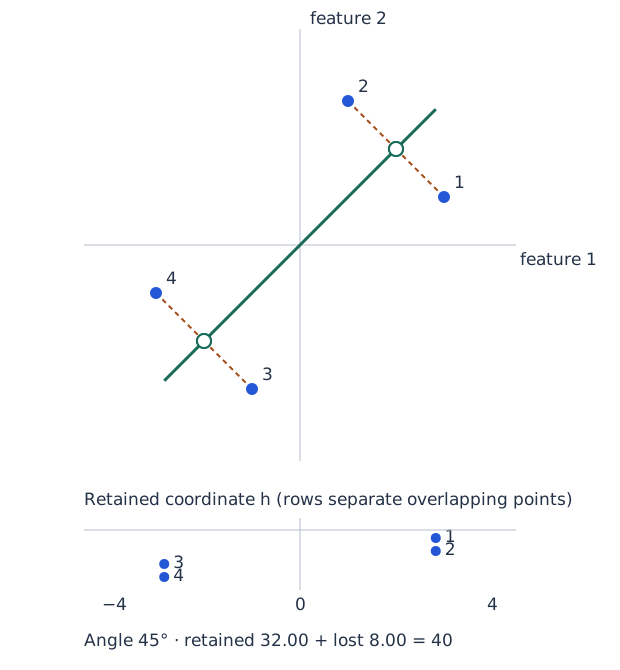
Filled blue circles: observations; open green circles: projections; dashed orange segments: lost residuals. Point numbers identify the same observations in both views. Move the angle with the slider or arrow keys; the data stay fixed.

Figure 2: Rotating one line trades retained variation against reconstruction error. Filled blue circles are fixed centered observations, open circles are their projections, and dashed orange segments are residuals. The lower strip shows the retained scalar coordinates. At 45°, the retained sum of squares is 32 and the residual sum is 8; their total stays 40. Original synthetic course calculation.

Use Figure 2 to compare the same observations under several candidate directions. The line controls both the retained coordinates and the reconstructed points. The residual segments show what is lost. The numerical values come from a four-observation example that we will trace completely after the derivation.

Changing coordinates before discarding information

There are two different operations inside dimension reduction: describe the same observations in a new coordinate system, then retain only some of those coordinates. Figure 3 separates them using 450 synthetic observations in common arbitrary units. Colors follow each point’s second principal score through every panel; three numbered observations make individual points easy to track. The colors do not denote classes.

Figure 3: Centering translates the cloud, changing to principal coordinates re-expresses it, and dropping PC2 removes information. Both principal directions are shown before reduction.

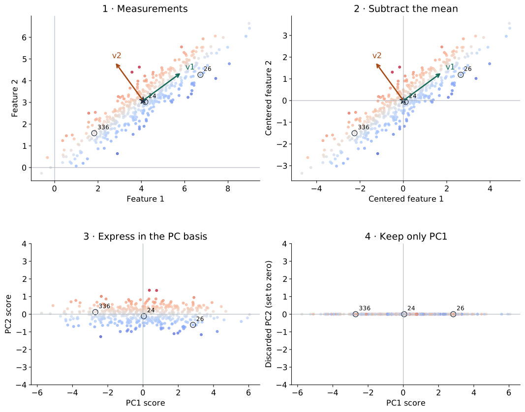
The star marks the mean. Subtracting it translates every point by the same amount. The two perpendicular arrows identify a new coordinate system: the first along the long direction of the cloud, the second across it. A point’s signed positions along these directions are its PC1 and PC2 scores. Keeping both scores describes the same point without losing information.

The last panel retains only PC1. Points separated across the cloud can now coincide on the line. Changing the coordinate system is reversible; discarding one coordinate generally is not. These are the coordinate operations in the two algorithms. We can now derive which directions minimize their reconstruction error.

The geometry behind the algorithms

For one retained direction, the matrix operations in the algorithms become a pair of vector calculations. With \(n\) training observations, the fitted mean and centered observations are

\[ \bar x=\frac1n\sum_{i=1}^n x_i,\qquad \widetilde x_i=x_i-\bar x. \]

Centering subtracts the mean of each feature separately, so \(\sum_i\widetilde x_i=0\). The matrix \(X_c\in\mathbb R^{n\times D}\) has rows \(\widetilde x_i^\top\). Centering lets a line through the origin describe variation around the average observation. Later, adding \(\bar x\) will restore the original location.

Let \(v\in\mathbb R^D\) be a unit direction, \(v^\top v=1\). Its length is fixed so that changing the scale of \(v\) cannot artificially enlarge a coordinate. The retained coordinate and reconstructed observation are

\[ h_i=v^\top\widetilde x_i,\qquad \widehat x_i=\bar x+h_i v. \]

The scalar \(h_i\) is a signed distance along \(v\). Multiplying it by \(v\) places a point back on the line; adding the mean returns to the original coordinate system. The residual \(e_i=x_i-\widehat x_i=\widetilde x_i-h_iv\) is what the representation loses. Its dot product with the line direction is zero:

\[ v^\top e_i=v^\top\widetilde x_i-h_i v^\top v=h_i-h_i=0. \]

Thus reconstruction is an orthogonal projection: among points on this line, it is closest to the observation in Euclidean distance. The remaining question is why the covariance eigenvector selects the best line.

Why keeping variance also minimizes error

Choose a unit direction to minimize the summed squared reconstruction loss:

\[ L(v)=\sum_i\|\widetilde x_i-(v^\top\widetilde x_i)v\|^2, \qquad v^\top v=1. \]

The reconstruction relative to the mean, \(h_iv\), is perpendicular to the residual \(e_i\). Pythagoras therefore gives

\[ \|\widetilde x_i\|^2=h_i^2+\|e_i\|^2. \]

Add over the observations. The left-hand side depends only on the fixed centered data. Increasing the retained sum \(\sum_i h_i^2\) decreases the residual sum by exactly the same amount. Because the centered coordinates satisfy \(\sum_i h_i=0\), their empirical variance with denominator \(n\) is \(n^{-1}\sum_i h_i^2\). The line with maximum projected variance is the line with minimum squared reconstruction error. This equivalence uses orthogonal projection and squared Euclidean error.

The dataset’s total squared length is fixed. We can therefore solve either problem: minimize the residual sum or maximize the retained sum. Covariance will let us express the retained quantity directly as a function of the chosen direction.

Why covariance eigenvectors solve the problem

For a candidate direction, substitute \(h_i=v^\top\widetilde x_i\):

\[ \frac1n\sum_i h_i^2 =\frac1n\sum_i v^\top\widetilde x_i\widetilde x_i^\top v =v^\top C v. \]

PCA maximizes this quantity subject to \(v^\top v=1\). To see how eigenvectors enter, introduce a constraint multiplier \(\lambda\) and differentiate \(v^\top Cv-\lambda(v^\top v-1)\). Symmetry of \(C\) gives

\[ 2Cv-2\lambda v=0,\qquad Cv=\lambda v. \]

Multiplying the stationary-direction equation on the left by the unit vector’s transpose shows \(v^\top Cv=\lambda\): the eigenvalue is the variance along that direction. A symmetric covariance matrix has an orthonormal eigenbasis with nonnegative eigenvalues. Expanding a unit candidate in that basis makes its variance a weighted average of eigenvalues, with weights equal to squared expansion coefficients. Its largest possible value is therefore the largest eigenvalue.

Some software reports covariance eigenvalues with denominator \(n-1\). Relative to the \(1/n\) convention, that multiplies eigenvalues by \(n/(n-1)\) and leaves directions and explained-variance ratios unchanged. Reversing an eigenvector’s sign also leaves reconstruction unchanged: both its coordinates and direction reverse. Equal eigenvalues allow multiple equally good bases inside the tied eigenspace.

Several coordinates form a subspace

Sort the eigenvalues \(\lambda_1\ge\cdots\ge\lambda_D\ge0\) and put the first \(d\) unit eigenvectors into the columns of \(V\in\mathbb R^{D\times d}\). They satisfy \(V^\top V=I_d\). Encoding and reconstruction are

\[ H=X_cV\in\mathbb R^{n\times d},\qquad \widehat X=\mathbf1_n\bar x^\top+HV^\top \in\mathbb R^{n\times D}. \]

The vector \(\mathbf1_n\) contains \(n\) ones, so the first term repeats the mean in every row. The encoder takes coordinates along the selected directions; the decoder adds their contributions and restores the mean. A principal direction is a vector in input space; a principal-component score is an observation’s coordinate along it. Neither is an original feature in general.

The covariance of the retained training scores is shown below; \(\operatorname{diag}\) places the listed values on the diagonal and zeros elsewhere.

\[ \frac1n H^\top H=V^\top C V =\operatorname{diag}(\lambda_1,\ldots,\lambda_d). \]

Thus each score’s variance is its eigenvalue, and different principal scores have zero empirical covariance. This is what the coordinate-change picture accomplishes: joint linear variation becomes variation along separate axes. Zero covariance still does not establish independence, as the recap’s squared-feature example showed.

Orthogonality gives the same energy identity for matrices:

\[ \|X_c\|_F^2=\|X_cV\|_F^2+ \|X_c-X_cVV^\top\|_F^2. \]

The squared Frobenius norm, \(\|A\|_F^2=\sum_{i,j}A_{ij}^2\), adds squared entries. With the \(1/n\) covariance convention, the retained sum is \(n\sum_{j=1}^d\lambda_j\) and the residual sum is \(n\sum_{j=d+1}^D\lambda_j\). For a positive total variance, the explained-variance ratio is

\[ \frac{\sum_{j=1}^d\lambda_j}{\sum_{j=1}^D\lambda_j}. \]

Retaining all nonzero-variance directions reconstructs the centered training data exactly. With fewer directions, the discarded eigenvalues quantify the training reconstruction error. A full basis also reconstructs new observations exactly, while retaining only the training-data span need not preserve a new observation outside that span.

A scree plot displays eigenvalues in order; cumulative explained variance shows what each additional coordinate retains. Retaining more directions increases the available variation and decreases reconstruction error, but also increases the coordinate count. Choose \(d\) according to the purpose: a visualization budget, an acceptable reconstruction error, or validated performance on a downstream task. An 80% ratio describes squared variation in the chosen feature units; it does not mean 80% of semantic information has survived.

A complete worked example

Now apply both algorithms to four observations with two features in common units. These are the observations used in the projection control. The panels carry one dataset through fitting, encoding, and reconstruction. Each panel gives the formula and its result.

1 · Observations

\[ X=\begin{pmatrix}5&3\\3&5\\1&-1\\-1&1\end{pmatrix} \in\mathbb R^{4\times2}. \]

\(n=4,\quad D=2,\quad d=1\).

2 · Center

\[ \bar x=\frac1n\sum_i x_i =\begin{pmatrix}2\\2\end{pmatrix}, \] \[ X_c=X-\mathbf1_n\bar x^\top =\begin{pmatrix}3&1\\1&3\\-1&-3\\-3&-1\end{pmatrix}. \]

3 · Covariance

\[ C=\frac1nX_c^\top X_c =\begin{pmatrix}5&3\\3&5\end{pmatrix}. \]

4 · Principal directions

\[Cv_j=\lambda_jv_j.\]

\[ v_1=\frac1{\sqrt2}\begin{pmatrix}1\\1\end{pmatrix},\quad\lambda_1=8, \] \[ v_2=\frac1{\sqrt2}\begin{pmatrix}1\\-1\end{pmatrix},\quad\lambda_2=2. \]

5 · Retain and encode

\[V=v_1,\qquad \frac{\lambda_1}{\lambda_1+\lambda_2}=80\%.\]

\[ H=X_cV =\begin{pmatrix}2\sqrt2\\2\sqrt2\\-2\sqrt2\\-2\sqrt2\end{pmatrix} \in\mathbb R^{4\times1}. \]

6 · Reconstruct and check

\[ \widehat X=HV^\top+\mathbf1_n\bar x^\top =\begin{pmatrix}4&4\\4&4\\0&0\\0&0\end{pmatrix}. \]

\[L=\|X-\widehat X\|_F^2=8,\] \[\mathrm{MSE}=\frac{L}{nD}=1.\]

Figure 4: PCA from two features to one coordinate and back: read left to right, then down. One retained direction preserves 80% of training variation; reconstruction has per-feature MSE 1. Original course calculation in common arbitrary units, using covariance denominator \(n=4\).

Interpreting the numbers

Figure 4 separates shared fitted quantities from per-observation information: \(C\) describes variation in the dataset, \(V\) specifies the retained direction, and each row of \(H\) describes one observation. Follow the first row through all six panels; then explain why the first two rows reconstruct identically even though their original measurements differ.

The fixed total centered squared length is \(40\). The chosen diagonal direction retains \(32\) and loses \(8\). A horizontal projection would retain \(20\) and lose \(20\): the first centered feature is kept and the second is discarded. The diagonal improves reconstruction with the same one-coordinate budget.

Check the units of the reported error. Total squared error \(8\), mean squared distance per observation \(8/4=2\), and per-feature MSE \(8/(4\cdot2)=1\) describe the same reconstruction. The mean and basis remain shared fitted quantities in addition to the observation scores. Recovering all feature columns does not mean all their information survived compression.

Check the example in NumPy

The following NumPy calculation implements Algorithm 1 using a symmetric eigensolver, then applies Algorithm 2. The assertions check the covariance, retained variance, and reconstruction error for our four observations.

In computation, singular value decomposition (SVD) of \(X_c\) can obtain the same directions without explicitly forming \(X_c^\top X_c\). If \(X_c=US R^\top\), the columns of \(R\) are principal directions and the covariance eigenvalues are the squared singular values divided by \(n\). The two algorithms describe the same representation whichever numerical route is used.

import numpy as np

X = np.array([[5., 3.], [3., 5.], [1., -1.], [-1., 1.]])
mean = X.mean(axis=0)
Xc = X - mean
C = Xc.T @ Xc / len(X)
eigenvalues, directions = np.linalg.eigh(C)  # ascending order
order = np.argsort(eigenvalues)[::-1]
eigenvalues = eigenvalues[order]
V = directions[:, order[:1]]                # (D, d) = (2, 1)
H = Xc @ V                                 # (n, d) = (4, 1)
Xhat = mean + H @ V.T                       # broadcast mean to rows
assert np.allclose(C, [[5, 3], [3, 5]])
assert np.allclose(eigenvalues, [8, 2])
assert np.allclose(((X - Xhat) ** 2).sum(), 8)
assert np.allclose(H.T @ H / len(X), [[8]])

For an experiment on new observations, fit preprocessing and PCA on training data, use validation data to choose the retained dimension or other settings, and evaluate the frozen choice on test data. The two algorithms specify which fitted quantities must stay fixed.

When a projection keeps the groups apart

We have checked reconstruction numerically. Now ask whether a retained coordinate can also preserve visible groups. Consider 540 observations forming three compact groups in Figure 5. The colors and marker shapes identify the synthetic generating groups; they are revealed for interpretation and never enter the PCA fit.

Figure 5: Keeping either original feature merges two groups; the first principal coordinate keeps all three groups in separate intervals in this constructed example. The vertical rows in the coordinate panels are annotations for legibility, not additional learned dimensions.

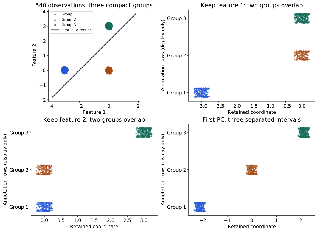
Start with the top-left panel. Two groups share approximately the same first coordinate; another pair shares approximately the same second coordinate. Dropping either feature merges a pair. The oblique principal direction combines both features. Here the group centers spread out along that direction enough for their projected intervals to remain separate. The larger spread between groups is aligned with the direction PCA wants to keep.

Here a linear representation serves both compression and group inspection: the three projected score intervals do not overlap. PCA produces coordinates; a separate clustering method would assign groups. In this dataset’s geometry, the separation of groups aligns with large variance. We will compare this success with image observations and curved structures next.

From a pixel vector to a reconstructed image

Images extend the same two algorithms to hundreds of features, letting us inspect what reconstruction preserves beyond a synthetic point cloud. We use MNIST handwriting at its original \(28\times28\) resolution, giving \(D=784\) pixel measurements per image (LeCun et al. 1998). Intensities are divided by the known constant 255. The official Torchvision MNIST loader documentation describes the source files.

For this separate textbook illustration, shuffle the 60,000 official training-image IDs with seed 42. Use the first 6,000 to fit the mean and principal directions and the next 1,000 as a validation set for reconstruction checks. These validation images are held out, meaning excluded from fitting the mean and directions. The official test partition is untouched. This is an image split, not an experiment on unseen writers, and it is independent of the tutorial’s split. No labels enter the split, fitting, or selection of displayed examples. The five displayed rows are simply the first five held-out IDs after the shuffle.

Figure 6: The average training image is a baseline reconstruction. Principal directions are signed pixel patterns; red and blue indicate opposite contributions, using one shared scale across directions.

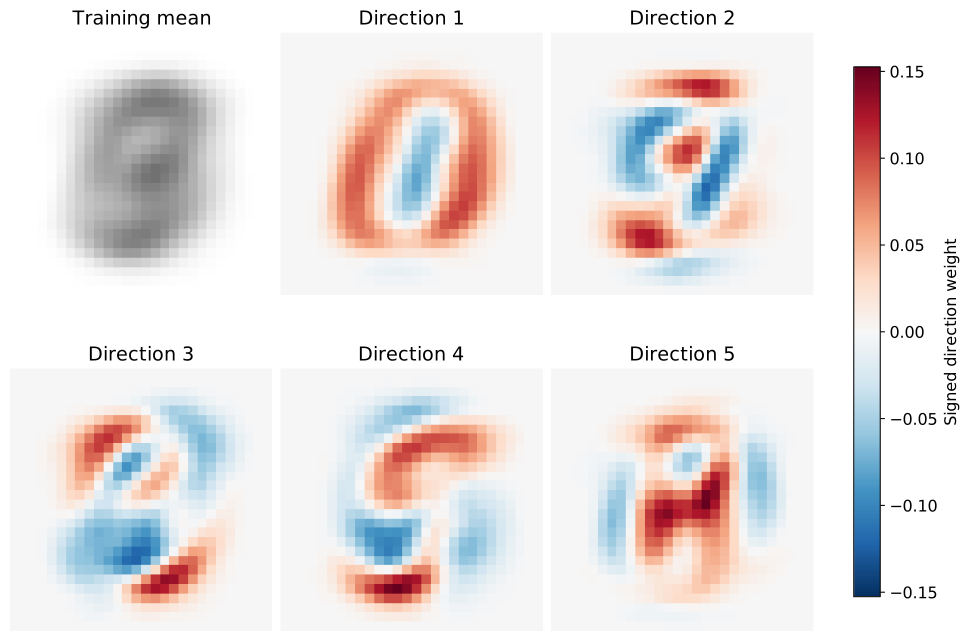
In Figure 6, the mean is an image, but a direction is a vector of signed weights. A positive score adds its positive-weight pixels and subtracts its negative-weight pixels; a negative score reverses those changes. Reconstructing with \(d\) coordinates forms a weighted sum of \(d\) such patterns and adds the mean. The directions need not look like complete digits or represent named visual concepts.

Figure 7: The same five held-out images reconstructed with progressively more principal coordinates. Every row uses the same observation and fitted basis.

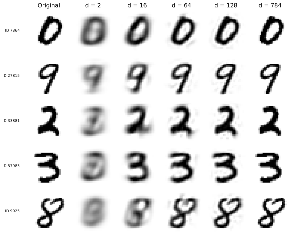
Read Figure 7 from left to right. Two coordinates give each of these images only two adjustable coefficients around the shared mean. More coordinates allow finer stroke differences. At 784 coordinates the full orthonormal basis reconstructs any 784-dimensional input to numerical precision; this endpoint provides a check, with no coordinate compression. The display uses the same fixed grayscale range, \([0,1]\), in every panel. Pixel values outside that range are saturated for display only; numerical errors are computed from the unmodified reconstructions.

Figure 8: Training explained variance rises as held-out reconstruction error falls. The curves summarize different data and different quantities.

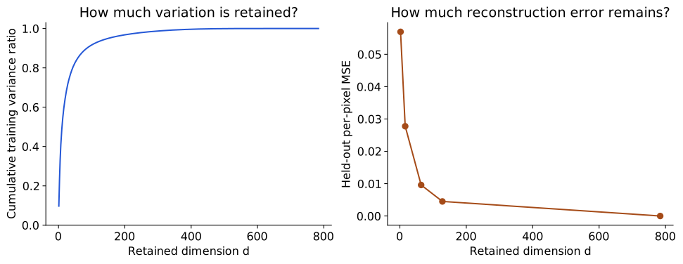
Figure 8 connects the pictures to measurements. With 64 coordinates, the fit retains about 86.4% of training variation and has mean squared pixel error about 0.00959 across the 1,000 held-out images. With 128 coordinates these values are about 93.8% and 0.00450. All five dimensions were specified for illustration; we have not selected a winning dimension or measured recognition accuracy.

Reconstruction error decreases even on this fixed held-out set because we extend one nested orthonormal basis: each added direction can only remove another squared residual component. This algebraic property does not establish semantic usefulness or performance on a different population. Sixty-four coordinates instead of 784 reduce the per-image coordinate count to about 8.2% of the original; the shared mean and basis, their numerical precision, and storage overhead must also be counted in a storage comparison.

What does a two-coordinate image map show?

Compression gave us reconstructed images. Now use just the first two coordinates as a map: one point per image, with its PC1 score on the horizontal axis and PC2 score on the vertical axis. Figure 9 uses the same 1,000 held-out observations and the same fitted basis as the reconstructions. The five thumbnails are the same five images already displayed, selected by their fixed held-out order.

Figure 9: MNIST in the first two principal coordinates. Thumbnails connect image observations to points; labels added after fitting reveal substantial overlap.

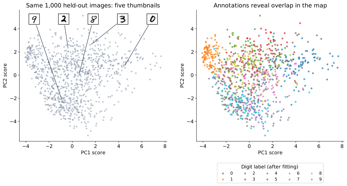
Each thumbnail’s connector ends at the image’s coordinates; its offset on the page is only for legibility. Trace a thumbnail to its point, then locate that point in the annotated panel. A region contains visibly different digits: different images can have similar values of these two weighted pixel sums. The map retains about 16.7% of this fit’s training variation; the other 782 coordinates are absent. That percentage quantifies retained variation, while the annotations separately show class overlap.

Digit annotations are loaded after the basis and map coordinates have been computed. The right panel reveals which categories occupy similar regions; it does not alter their positions. This is a visual diagnostic of a fixed representation. PC1 and PC2 are weighted pixel combinations, so moving right cannot be identified with a named property such as “more curved” without examining the corresponding images and direction weights. Nearby map points have similar retained coordinates, but may differ substantially in the discarded directions. We will reuse this distinction when comparing PCA with a neighborhood-based map.

Fitting once, transforming many observations

The numerical work has two stages. Fitting estimates the training mean and directions. Transforming applies the fixed rule to an observation: subtract that mean and take \(d\) dot products, each involving \(D\) measurements. For \(m\) new observations, this dense calculation requires work proportional to \(mDd\); with \(D,d\) fixed, it grows linearly with the number of observations. No iterative search for each new point’s position is needed.

Fitting has a different cost. Explicitly constructing the \(D\times D\) covariance matrix requires work proportional to \(nD^2\), and a full dense eigendecomposition scales cubically in \(D\). The SVD route avoids constructing that covariance matrix; the best numerical approach depends on the matrix dimensions and how many directions are required. For large problems, approximate truncated or incremental methods can be useful. The scikit-learn decomposition guide explains the available solver families. These explicit operations make PCA a useful computational baseline. Its fitting cost depends on both sample count and feature dimension, as well as the solver.

The input measurements need not be pixels. Suppose a frozen neural encoder gives each observation a representation \(h_i\in\mathbb R^d\). We can fit another PCA basis to training representations, then project new encoder outputs using that fixed representation mean and basis. To avoid confusing the learned representation with the new map, call its two displayed coordinates \(s_i\in\mathbb R^2\). PCA then asks which linear combinations of encoder features vary most; it does not change the encoder or make those directions semantic factors automatically.

An explained-variance ratio quantifies variation in the chosen feature units. It can help us judge how much a two-coordinate view omits, while downstream evaluation addresses whether the features support a particular task. This gives PCA two distinct roles in our story: a representation learned directly from measurements, and a tool for inspecting representations learned by another model.

When the retained variation misses the useful structure

A pair of spirals makes the linear restriction visible. Each arm bends through the plane, so the distinction between arms depends on location around the curves. A single straight projection adds together points from different turns. In the top row of Figure 10, many observations on different arms receive similar scores. One coordinate has not unrolled the curves.

Figure 10: Curved geometry can be lost under linear projection, and even a straight separating boundary can depend on a direction PCA discards. Annotation rows separate markers only for display.

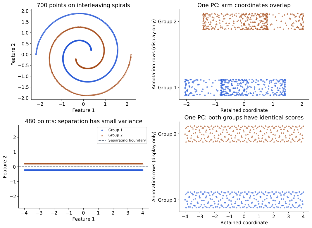
Keeping both principal coordinates in this two-dimensional spiral example would preserve the whole plane through a rotation or reflection. The limitation illustrated here is reducing the data to one linear coordinate while preserving the arm distinction. A nonlinear boundary by itself is not evidence that every PCA representation is useless. The question is whether the retained linear subspace preserves the relationships needed for the intended task.

The bottom row provides a second, different failure. Two horizontal strips are separated perfectly by the straight boundary “feature 2 equals zero.” Their horizontal variation is much larger than their vertical separation. PCA therefore keeps the horizontal coordinate, and both groups have identical projected score sets. Linear separability in the original space does not guarantee separation after PCA. Compare this with the successful three-group example: the alignment between high variance and the useful distinction is what changed.

The examples return us to the objective. PCA chooses directions using squared variation in the chosen feature units. It succeeds when that variation follows the structure we want to preserve; it can discard a small but useful distinction or fail to express a curved relationship compactly. Large outliers can also rotate the fitted directions because squared deviations receive large weight.

What to carry forward. The fitted mean and basis define the encoder; retained scores describe individual observations; the decoder reconstructs by expanding those scores and restoring the mean. Orthogonality connects retained variance to reconstruction error. Whether the representation supports grouping or recognition requires evidence beyond that objective.

Pause and interpret. In the four-point example, trace \((5,3)^\top\) through both algorithms. Which step loses information? Why does reversing the retained direction preserve reconstruction? Then compare the separated groups, the MNIST map, and the spirals: what does each show about the relationship between high variance and useful structure?

If reconstruction needs a curved representation, we can learn a nonlinear encoder and decoder. If our purpose is a picture of local relationships, we can instead change the mapping objective. That second question leads to t-SNE.

t-SNE: a map of local relationships

The PCA image map gives every digit two coordinates, but several digit categories overlap. Its objective preserves squared variation. What if our purpose is to inspect which observations resemble one another locally? We can give nearby observations a strong preference to remain neighbors on the page, while allowing other relationships to change.

t-distributed stochastic neighbor embedding (t-SNE) makes a map by comparing probabilities assigned to pairs of observations. We will build that comparison from distances, first around one anchor observation and then across the dataset. The construction follows van der Maaten and Hinton’s method (Maaten and Hinton 2008). Their paper uses \(y_i\) for map coordinates; here we write \(v_i\in\mathbb R^2\), reserving \(y_i\) for external task labels. The map coordinates are fitted variables, not the output of a PCA basis.

What the procedure will do

The observations \(x_i\in\mathbb R^D\) and their input metric stay fixed. Each observation gets a map point \(v_i\in\mathbb R^2\). The procedure moves those map points so that pairs assigned high probability in the input space also tend to receive high probability in the map.

Step	Operation	Result
1 · Define resemblance	Choose observations, preprocessing, and an input distance.	A declared geometry for the input observations.
2 · Weight neighbors	Around each observation, convert squared distances to Gaussian weights and normalize. Select its bandwidth to match a chosen perplexity.	Conditional neighbor probabilities \(p_{j\mid i}\).
3 · Combine the views	Average the two directed probabilities for each pair, with dataset normalization.	Symmetric input affinities \(P_{ij}\).
4 · Initialize a map	Give the same observations small initial coordinates; define Student-kernel map affinities.	Coordinates \(v_i\) and probabilities \(Q_{ij}\).
5 · Fit the map	Move coordinates to reduce \(L=\sum_{i\ne j}P_{ij}\ln(P_{ij}/Q_{ij})\).	A map fitted jointly for these observations.
6 · Inspect and check	Compare declared settings and neighborhood identities; add external annotations after fitting.	Evidence about what the map preserves.

This is the overall algorithm. Next we will open each probability calculation. In particular, a Gaussian density height, an unnormalized weight, and a discrete neighbor probability have different meanings.

From a distance to a neighbor probability

Choose an anchor observation \(x_i\). Let \(\delta_{ij}=\|x_i-x_j\|\) be its Euclidean distance to another observation. We want a positive weight that decreases smoothly as distance grows. A Gaussian-shaped kernel supplies

\[ w_{j\mid i}=\exp\!\left(-\frac{\delta_{ij}^2}{2\tau_i^2}\right), \qquad j\ne i, \]

where the bandwidth \(\tau_i>0\) sets the local scale. Small distances relative to \(\tau_i\) get large weights; distances many bandwidths away get small ones. Exclude the anchor itself: otherwise its zero distance would give it a weight of one for being its own neighbor.

The weights do not yet sum to one. Normalize over the other observations:

\[ p_{j\mid i}=\frac{w_{j\mid i}}{\sum_{k\ne i}w_{k\mid i}}, \qquad p_{i\mid i}=0,\qquad\sum_{j\ne i}p_{j\mid i}=1. \]

Imagine choosing one other observation according to these masses. A nearby candidate is more likely to be chosen. This is the meaning of “stochastic neighbor”: the formula defines a distribution over candidate observation IDs. It does not assert that the data were drawn from a Gaussian population.

In one dimension, evaluating a normal density with mean \(x_i\) and standard deviation \(\tau_i\) gives the same relative weights. The density’s normalizing factor is common to all candidates for this anchor and cancels when we normalize over them. In \(D\) dimensions the same reasoning uses an isotropic Gaussian kernel. We retain the exponential factor and normalize over the finite candidate set.

Figure 11: One anchor, four fixed candidates: widening the Gaussian changes their relative weights and the normalized masses below it. Orange highlights one candidate’s density height and probability bar. The bell curve is a density; the bars form a discrete distribution over observation IDs. Original synthetic course calculation with a static bandwidth-1 fallback.

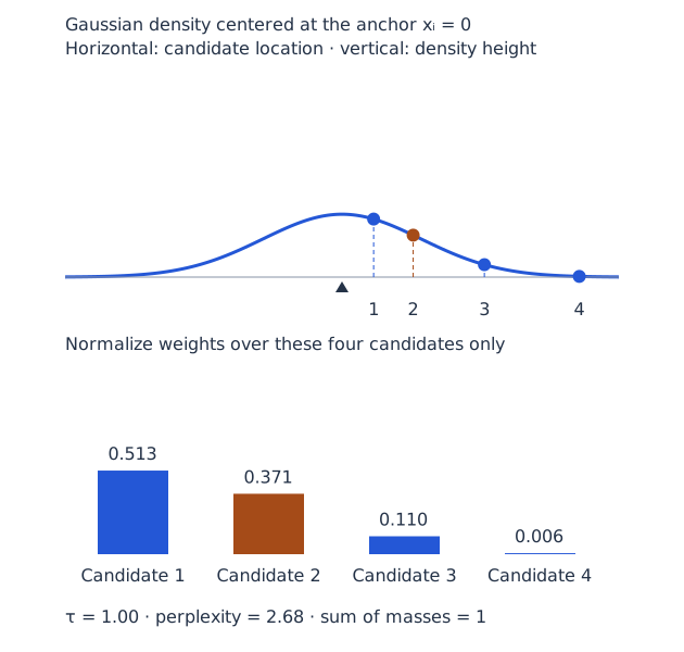
In Figure 11, move the bandwidth slider and follow candidate 2. A narrow kernel concentrates the distribution on the closest candidate; widening it gives the farther candidates more mass. The top marker is a height, not an interval probability. No shaded area under the curve is needed to obtain the bars: each bar comes from a candidate’s weight divided by the sum of all candidate weights. This uses the same point-and-distribution reading approach as Week 07, with a different normalization question.

The inputs in this illustration are one-dimensional only so we can draw them. In an image dataset the distances are calculated between pixel vectors or encoder representations, not between digit IDs.

Perplexity chooses the local scale

How wide should each Gaussian be? A fixed bandwidth can make nearly everyone look distant in a sparse region and nearly everyone look close in a dense region. t-SNE instead chooses a bandwidth separately for each anchor to reach a specified perplexity.

For the conditional distribution around \(i\), define its entropy and perplexity using natural logarithms:

\[ \mathcal H_i=-\sum_{j\ne i}p_{j\mid i}\ln p_{j\mid i}, \qquad \operatorname{Perp}_i=\exp(\mathcal H_i). \]

If exactly \(k\) candidates have equal probability \(1/k\) and all other probabilities are zero, then \(\mathcal H_i=\ln k\) and perplexity is \(k\). For unequal masses it acts as an effective neighborhood size, not a literal count of selected neighbors or a requested number of clusters.

Increasing \(\tau_i\) generally spreads mass over more candidates and raises perplexity. A one-dimensional search for the bandwidth can therefore match the target, up to tolerance and constraints from tied distances. The same target can require different bandwidths around different observations. For \(n\) observations, the theoretical effective count cannot exceed \(n-1\); attainable lower limits also depend on distance ties. Choose feasible perplexities relative to the sample size.

The slider displays the achieved perplexity for its manually chosen bandwidth. A complete t-SNE fit runs the relationship in the other direction: you specify perplexity, and the algorithm finds the bandwidths. This is why increasing perplexity does not simply enlarge every cluster on the screen by a predictable factor.

A compact neighbor calculation

At bandwidth \(\tau_i=1\), take the four candidate distances from the interactive figure. The formula and its results are:

Quantity	Result
Distances \(\delta_{ij}\)	\((0.4,\ 0.9,\ 1.8,\ 3.0)\)
Weights \(w_{j\mid i}=\exp(-\delta_{ij}^2/2)\)	\((0.9231,\ 0.6670,\ 0.1979,\ 0.0111)\)
Masses \(p_{j\mid i}=w_{j\mid i}/\sum_k w_{k\mid i}\)	Approximately \((0.5131,\ 0.3707,\ 0.1100,\ 0.0062)\)
Perplexity \(\exp(-\sum_jp_{j\mid i}\ln p_{j\mid i})\)	Approximately \(2.68\)

The probabilities are dimensionless. Dividing all weights by the same positive constant would leave them unchanged. Conversely, changing the input metric or relative feature scaling changes distances and can change the neighbor distribution: the method needs a meaningful notion of resemblance before it can preserve one.

SNE supplies the idea; t-SNE changes the map model

The earlier stochastic neighbor embedding (SNE) idea compares conditional neighbor distributions in the input and map spaces. A Gaussian kernel can be used in both. t-SNE makes two changes we need to understand: it uses symmetric joint affinities for pairs, and a heavy-tailed Student kernel in the map. These choices are part of its geometry and optimization, not simply a way to avoid computing exponentials.

First combine the input distributions:

\[ P_{ij}=\frac{p_{j\mid i}+p_{i\mid j}}{2n},\qquad P_{ii}=0. \]

A dense and a sparse observation can assign each other different conditional probabilities, so averaging makes the pair description symmetric. Because there are \(n\) conditional distributions, each summing to one, division by \(2n\) gives

\[ P_{ij}=P_{ji},\qquad \sum_{i\ne j}P_{ij}=1. \]

We sum over ordered pairs: \((i,j)\) and \((j,i)\) both appear. The entries of \(P\) are probabilities of pairs of observation IDs, not probabilities of digit classes.

Now place observations in the map, with rows \(v_i^\top\) in a coordinate matrix of shape \(n\times2\). Define

\[ a_{ij}=\frac1{1+\|v_i-v_j\|^2},\qquad i\ne j, \] \[ Q_{ij}=\frac{a_{ij}}{\sum_{r\ne s}a_{rs}},\qquad Q_{ii}=0. \]

The indices \(r,s\) run over observations; \(a_{ij}\) denotes an unnormalized map weight. This Student kernel has one degree of freedom. As with \(P\), the map affinities are symmetric and sum to one over ordered off-diagonal pairs. Unlike the input construction, their normalization is global across pairs, and there is no separately fitted bandwidth for each map point.

Why a heavy-tailed map kernel?

Many moderately close neighbors in a high-dimensional space can be difficult to arrange around one point in a two-dimensional map. The amount of surrounding space grows differently with radius in different dimensions. Trying to keep all these relationships can crowd points together. A two-dimensional map cannot generally preserve every relationship exactly.

Figure 12: The Student kernel keeps more weight at larger distances than a Gaussian kernel. The logarithmic panel reveals the tail difference.

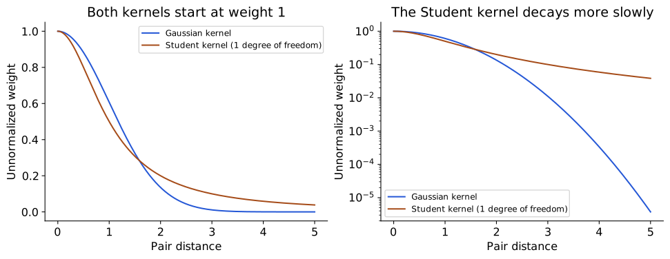
The heavy tail in Figure 12 allows a moderate pair affinity to be represented at a larger map distance than a rapidly decaying Gaussian weight would allow, easing the pressure to crowd points centrally. The kernel also changes the forces used in fitting. It does not make map distances globally calibrated, guarantee that every neighborhood survives, or establish that visible islands are true categories. The plotted curves compare raw kernel shapes; the actual \(Q_{ij}\) additionally depends on the positions of every map point through its denominator.

Match the pair distributions with KL

Hold the input affinities \(P\) fixed and vary the map coordinates through \(Q\). The objective is

\[ L= D_{\mathrm{KL}}(P\|Q) =\sum_{i\ne j}P_{ij}\ln\frac{P_{ij}}{Q_{ij}}. \]

This Kullback–Leibler divergence (KL) uses the same mathematical construction encountered in Week 07, but its outcomes here are pairs of observation IDs. It is not the VAE’s divergence between latent-variable distributions. KL is nonnegative for normalized distributions, is asymmetric, and is not a distance metric. Individual summands can be negative even though the total cannot.

Why this order, \(P\|Q\)? A pair with large input probability receives a large weight in the objective. Assigning it very small map probability is costly. Holding \(P\) fixed, minimizing KL is equivalent to minimizing \(-\sum P_{ij}\ln Q_{ij}\) because \(\sum P_{ij}\ln P_{ij}\) does not depend on the map. The criterion emphasizes recovering input-neighbor relationships; it does not minimize the difference between all original and displayed Euclidean distances.

To see where the update comes from, write \(Z=\sum_{r\ne s}a_{rs}\) and substitute \(Q_{ij}=a_{ij}/Z\):

\[ L=\underbrace{\sum_{i\ne j}P_{ij}\ln P_{ij}}_{\text{fixed}} -\sum_{i\ne j}P_{ij}\ln a_{ij}+\ln Z. \]

The last coefficient is one because \(\sum P_{ij}=1\). Differentiating the second term gives attraction weighted by \(P\); differentiating \(\ln Z\) supplies the corresponding term weighted by \(Q\). Symmetry counts each pair in both orders. Combining these terms gives

\[ \frac{\partial L}{\partial v_i} =4\sum_{j\ne i}(P_{ij}-Q_{ij}) \frac{v_i-v_j}{1+\|v_i-v_j\|^2}. \]

Read one term at a time. If \(P_{ij}>Q_{ij}\), the negative-gradient update attracts the pair. If \(P_{ij}<Q_{ij}\), it repels them. The inverse-distance factor comes from the Student kernel. Because moving one point changes the normalization of \(Q\), fitting is a coupled problem: the map is learned jointly, not by projecting each observation independently.

Watch optimization rearrange a map

Figure 13: A fixed pair distribution guides the same 90 observations through four stages of exact KL optimization. Labels mark synthetic generating groups and do not enter fitting.

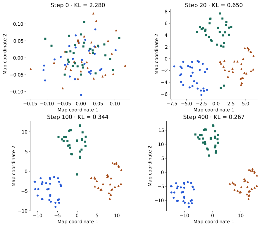
The observations in Figure 13 have three input features. We fix \(P\) at perplexity 8, initialize small random two-dimensional coordinates, and update those coordinates using the exact gradient above. A backtracking step rule accepts a step only when the unmodified KL decreases. Each snapshot displays the measured objective for the same input probabilities.

This is a transparent teaching optimizer. Library implementations use additional schedules and approximations; for example, early exaggeration temporarily increases attractive input-affinity terms, and momentum changes the update. Those intermediate iterations should not be interpreted as minimizing the same normalized KL at every step. A lower final KL establishes a better fit to this pair objective, not better classification or a uniquely correct picture. Compare neighbor identities and data examples as well as the displayed objective.

MNIST: same images, different map choices

Return to the same 1,000 held-out MNIST images already used in the PCA map. Here all 1,000 images participate jointly in fitting t-SNE coordinates; “held out” describes their role in fitting the earlier PCA basis, not their role in this map optimizer. We use their 784 scaled pixel intensities directly, Euclidean distance, no preceding PCA reduction, and no labels in fitting. This compares the objectives using the same observations and input representation.

Figure 14: Four t-SNE maps use identical MNIST images and raw-pixel distances. The first three change perplexity at fixed initialization seed; the fourth changes the seed at perplexity 30.

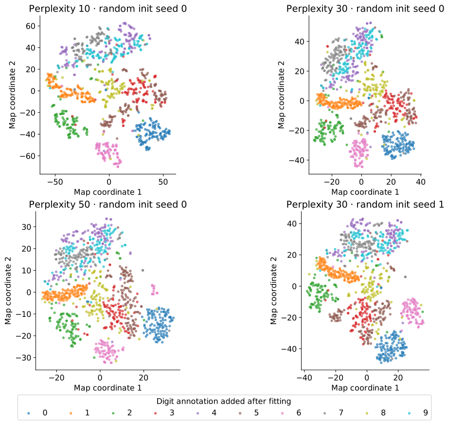
In Figure 14, colors reveal digit annotations only after fitting. Perplexity changes which neighborhood scale the input probabilities emphasize; random initialization changes the optimization path. These maps were all retained, with no label-based selection of a favorite run. They use scikit-learn 1.6.1, Barnes–Hut approximation, automatic learning rate, random initialization, and 1,000 iterations (scikit-learn developers, n.d.). The standard early-exaggeration schedule is left at its default. The generator records all settings and metrics.

Start by finding a group of one digit, then inspect places where colors mix. Compare the same observations by ID across runs, rather than asking whether islands have the same screen position. Rotation, reflection and translation do not change pairwise distances. Island area, apparent density, and gaps between separated islands do not provide direct estimates of those quantities in the input space. A visually isolated group also does not establish how many classes or clusters the data contain.

To put numbers beside the maps, take each image’s ten nearest neighbors in the original pixel space, excluding itself. Input-neighbor retention is the average fraction of those IDs also found among its ten nearest map neighbors. Trustworthiness additionally penalizes introduced map neighbors according to their ranks in the input space. Both depend on the chosen metric and neighborhood size. They audit local relationships; neither measures recognition accuracy or proves that all global relationships are correct.

Perplexity	Random seed	Input-neighbor retention (10)	Trustworthiness (10)
10	0	0.505	0.957
30	0	0.516	0.961
50	0	0.507	0.955
30	1	0.515	0.959

Using the result responsibly

Before changing perplexity or an optimizer setting, state what comparison will answer your question. Check several feasible neighborhood scales, inspect optimization diagnostics, and look for relationships stable across runs. Investigate ambiguous images rather than treating label agreement as the sole definition of useful structure. The caption must state the input representation and preprocessing: a map of encoder features answers a different question from a map of raw pixels.

A standard fitted t-SNE map also has a different deployment role from PCA. In the scikit-learn interface used here, fitting returns coordinates for the observations supplied to that fit; it does not provide PCA’s fixed transform rule for arbitrary future observations. Adding new observations and refitting can move the old points. Other methods and extensions can supply out-of-sample embeddings, but that requires an additional construction. Likewise, t-SNE does not provide a decoder for reconstructing a digit from an arbitrary map location.

Exact pair calculations have quadratic storage and pair-interaction costs in the observation count; approximate implementations reduce parts of that work. Actual runtime depends on sample count, input dimension, perplexity and solver settings. The Student kernel’s role is not a universal speed guarantee. For a quick linear view with a reusable transform, PCA remains a useful first comparison; t-SNE serves a different visualization objective.

What to carry forward. Distances define Gaussian neighbor weights; local normalization and perplexity define conditional probabilities; symmetrization gives \(P\); map positions define Student affinities \(Q\); KL moves the map toward the selected relationships. The resulting picture is evidence about that construction, interpreted with neighborhood checks and data examples.

Pause and interpret. In the bandwidth figure, which mark is a density height and which is a probability mass? If perplexity increases, which quantities are fitted again? Why can two credible maps place the same island on opposite sides of the page? Finally, what additional objective would be needed to turn a visual grouping into an explicit clustering?

TODO(instructor): review the new t-SNE prose, distribution control and experimental maps. UMAP remains an optional comparison for a later batch; its derivation is not included here.

Clustering: k-means and Gaussian mixture models

A map gives observations coordinates. A clustering gives them group assignments under a specified criterion. Suppose we want to organize a collection of objects without supplied category labels. We could choose a representative for each group and assign each object to its closest representative. But which representatives should we choose, and what does “closest” mean?

K-means makes those choices explicit: choose \(K\) centers and minimize squared distances to them. It produces a partition even when the observations do not contain naturally separated categories. We will understand that partition before moving to a probabilistic model with uncertain membership.

K-means: represent each group by its center

For \(n\) observations \(x_i\in\mathbb R^D\), choose \(K\) centers \(c_k\in\mathbb R^D\) and an assignment \(a_i\in\{1,\ldots,K\}\) for every observation. The objective is the within-cluster sum of squares, also called inertia:

\[ L(a,c)=\sum_{i=1}^n\|x_i-c_{a_i}\|^2. \]

A center is a vector in the same feature space as the observations; it need not be an observed example. If our features are pixels, a center can be an average image. If they are encoder outputs, the center is an average in that representation. The cluster count \(K\) is supplied, rather than discovered automatically by minimizing this objective.

The criterion defines a particular form of similarity: points in a group should lie close to one shared center under squared Euclidean distance. “Similar” therefore depends on which features and units we provide. Cluster IDs have no intrinsic ordering or category meaning: exchanging IDs leaves the partition and objective unchanged (Bishop 2006, sec. 9.1).

Algorithm: assign, update, repeat

Input: a matrix \(X\in\mathbb R^{n\times D}\), a cluster count \(1\le K\le n\), an initialization policy, and a stopping rule. Output: fitted centers and assignments. The basic alternating procedure is commonly called Lloyd’s algorithm.

Step	Operation	Result
1 · Initialize	Choose \(K\) centers in the feature space.	Initial candidates \(c_1,\ldots,c_K\).
2 · Assign	\(a_i\leftarrow\arg\min_k\|x_i-c_k\|^2\) for every \(i\).	Each observation belongs to its nearest center.
3 · Update	\(c_k\leftarrow n_k^{-1}\sum_{i:a_i=k}x_i\), where \(n_k=\#\{i:a_i=k\}\).	Each nonempty center becomes its members’ mean.
4 · Repeat	Alternate assignment and update until assignments stabilize or a declared tolerance/cap stops the iterations.	A fitted partition and its measured objective.
5 · Compare starts	Run the declared initializations; compare final objectives on the same data and metric.	A less initialization-dependent choice of fit.

The teaching implementation breaks exact ties using the smallest center index. If a cluster becomes empty, it keeps the old center: the mean of an empty set is undefined. Other implementations may relocate empty centers; the policy is part of the algorithm. A center kept for an empty cluster contributes no current loss and may acquire members at a later assignment.

For a new observation, apply the same feature preprocessing and choose the closest saved center. This gives an assignment in the fitted partition without refitting all centers. It does not give the probability that the observation belongs to a semantic class. If fitting stops at a numerical tolerance or iteration cap, recompute final nearest-center assignments before reporting the partition, and state whether the centers also equal those final groups’ means.

Watch the two operations separately

Figure 15: The same 300 observations undergo exact Lloyd steps. Assignment changes the cluster color and marker shape; update moves the cross-shaped centers. Every displayed loss is calculated at a recorded endpoint, with no interpolation. Controls start paused; the static alternative shows the first six steps. Original synthetic course calculation.

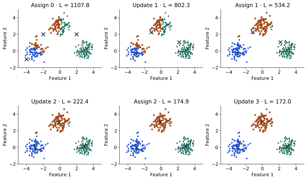
In Figure 15, move forward once from an assignment to an update. The observations stay fixed while each center moves to its group’s mean. Move forward again: the centers stay fixed while some observations change membership. These are different minimizations of one objective, not two names for the same operation.

The first centers were deliberately placed poorly to make reassignment visible. Their initial partition is a starting guess. The trace shows how optimizing it changes the groups; it does not establish that these are the only meaningful groups in the observations.

Why neither exact step increases the objective

When the centers are fixed, the contribution of observation \(i\) is \(\|x_i-c_{a_i}\|^2\). Choosing the nearest center minimizes that term independently of all other assignments. Summing these independent choices cannot increase \(L\).

Now hold assignments fixed and examine one nonempty group. Its contribution is

\[ L_k(c_k)=\sum_{i:a_i=k}\|x_i-c_k\|^2. \]

Differentiating with respect to the center vector gives

\[ \nabla_{c_k}L_k=2n_kc_k-2\sum_{i:a_i=k}x_i. \]

Setting the derivative to zero gives the mean update in the algorithm. The Hessian is \(2n_kI_D\), positive definite for \(n_k>0\), so this is the group’s unique minimizer. Each exact step therefore decreases or preserves the same summed objective.

This is alternating optimization: minimize over assignments, then centers, with the other quantities fixed. The objective is bounded below by zero, but monotone improvement does not imply a globally best partition. With finite data, consistent tie handling and exact steps, the procedure reaches a stable configuration; practical tolerances and caps govern actual stopping. Initialization still matters because multiple stable configurations can exist.

A compact complete calculation

Take four one-dimensional observations and request two groups. Each row below gives a formula and its result; assignments index centers starting at one.

Stage	Formula and result
Observations and initial centers	\(x=(0,2,8,10)\); \(c=(0,2)\); \(K=2\).
Assign 0	\(a_i=\arg\min_k(x_i-c_k)^2\): \(a=(1,2,2,2)\); \(L=100\).
Update 1	\(c_k=n_k^{-1}\sum_{i:a_i=k}x_i\): \(c=(0,20/3)\); \(L=104/3\).
Assign 1	\(a=(1,1,2,2)\); \(L=152/9\).
Update 2	\(c=(1,9)\); \(L=4\).
Assign 2	\(a=(1,1,2,2)\) is unchanged; the fit is stable.

The assignments and centers are held fixed in different rows. Reporting only the final centers would hide how the second observation changes groups. Here the final partition is compact and intuitive, but that outcome follows from this dataset and \(K\), not merely from a decreasing training loss.

The same result can be checked with the explicit operations below. This short example checks the algorithm, rather than delegating its logic to a library call.

import numpy as np

x = np.array([0., 2., 8., 10.])[:, None]
centers = np.array([0., 2.])[:, None]
losses = []
for _ in range(10):
    assignment = ((x[:, None] - centers[None, :]) ** 2).sum(2).argmin(1)
    losses.append(((x - centers[assignment]) ** 2).sum())
    updated = np.array([
        x[assignment == k].mean(0) if np.any(assignment == k) else centers[k]
        for k in range(2)
    ])
    losses.append(((x - updated[assignment]) ** 2).sum())
    if np.allclose(updated, centers):
        break
    centers = updated
assert np.all(np.diff(losses) <= 1e-10)
assert np.allclose(centers[:, 0], [1., 9.])
assert np.isclose(losses[-1], 4.)

A grouping depends on the ruler and the start

Consider the four corners \((\pm3,\pm1)\) with \(K=2\). Splitting left/right gives centers \((\pm3,0)\) and total loss \(4\). Splitting top/bottom gives centers \((0,\pm1)\) and total loss \(36\). Both are stable Lloyd configurations: within either partition, updating means and then assigning again leaves the partition unchanged.

Figure 16: The same four observations support two stable starts, and changing a feature’s units changes the preferred partition. All panels show the original axes.

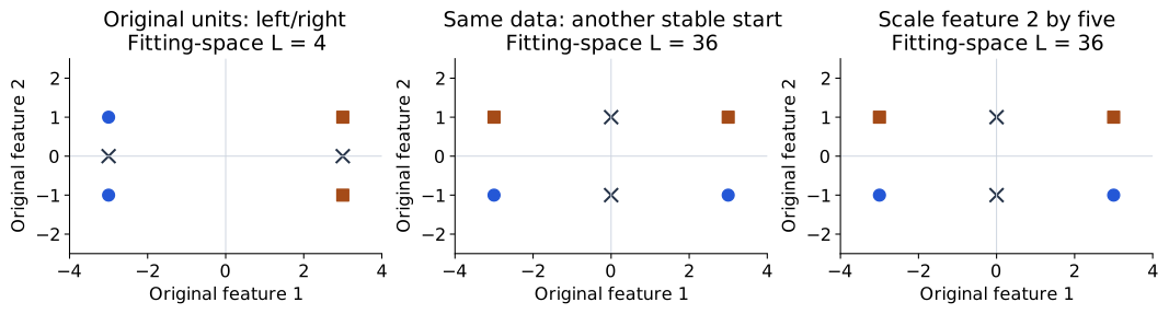
Now multiply the second feature by five before fitting. Squared distance becomes

\[ (x_1-x'_1)^2+25(x_2-x'_2)^2. \]

The left/right partition’s loss becomes \(100\), while the top/bottom partition’s loss remains \(36\). The observations drawn in Figure 16 have not moved on the original axes, but the metric used for fitting has changed. Losses across differently scaled spaces are not directly comparable quality scores. The relevant comparison is between candidate partitions within each chosen metric.

Initialization and scaling answer different questions. Trying several starts searches the same objective more thoroughly. Changing units changes the objective itself. Standardization may be appropriate when feature units should have comparable influence, using training statistics, but it is a modeling choice rather than a universal correction.

A spread-out initialization such as k-means++ helps reduce poor starting configurations; it does not guarantee that every run finds a global optimum. In reproducible comparisons, declare the initialization, number of restarts, seed and stopping settings. The scikit-learn clustering guide documents these implementation choices.

What shape of group does a center describe?

With centers fixed, points assigned to a center form its nearest-center region, or Voronoi cell. Under Euclidean distance these regions have linear boundaries between center pairs and are convex. This geometry favors compact groups; a curved connected structure can be split across several cells.

Figure 17: K-means partitions two curved arcs according to center distances. The generating groups are shown separately from the fitted assignments.

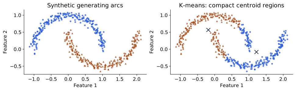
In Figure 17, both panels contain identical observations. The generating arc identity was not passed to k-means. The fitted partition is a reasonable solution to a nearest-center compactness objective, even though it does not recover the arcs. As with PCA, a limitation comes from a mismatch between the structure we want and the structure the objective rewards. Outliers can also move means substantially because squared residuals give distant points large influence.

Increasing \(K\) cannot increase the globally optimal training loss: additional centers can preserve or improve any existing fit. Thus choosing the lowest inertia over different \(K\) values alone favors more centers. Independent finite-restart runs can have nonmonotone measured losses because they may reach different local solutions. An elbow plot can help inspect diminishing improvements, but does not prove a natural cluster count.

Assess the partition using the purpose of grouping, stability across justified perturbations, and suitable diagnostics. A silhouette score compares within-group cohesion with distances to other groups under a chosen metric; it still favors particular geometries. External annotations can audit agreement after fitting, provided they were not used to select an apparently unsupervised result without disclosure. IDs are arbitrary, so use permutation-invariant comparisons. A map can illustrate assignments, but clustering t-SNE coordinates changes the metric and adds another optimization stage; visible islands do not validate the original-space clustering automatically.

Gaussian mixture models (GMM): soft membership

K-means makes an all-or-nothing choice for every observation. Near a boundary, two centers may be almost equally close, yet the output contains just one ID. Can a model express graded membership and describe the observations’ density as well?

A Gaussian mixture model (GMM) introduces an unobserved component index \(G_i\). Component \(k\) has probability mass \(\pi_k\), mean \(m_k\in\mathbb R^D\) and covariance \(\Sigma_k\in\mathbb R^{D\times D}\):

\[ P(G_i=k)=\pi_k,\qquad\pi_k\ge0,\qquad\sum_k\pi_k=1, \] \[ p(x_i\mid G_i=k)=\mathcal N(x_i;m_k,\Sigma_k), \qquad p(x_i)=\sum_k\pi_k\mathcal N(x_i;m_k,\Sigma_k). \]

The model says: choose a component, then draw an observation from its Gaussian. Summing over the unknown component gives the observable density. Unlike a class label, a component is a modeling device; several components can describe one semantic category, and one component can cover several categories. Covariance allows different spreads and orientations, subject to the chosen covariance family (Bishop 2006, sec. 9.2).

A point on two normal curves

Given fitted model parameters and an observed \(x_i\), Bayes’ rule gives its responsibility for component \(k\):

\[ r_{ik}=P(G_i=k\mid x_i) =\frac{\pi_k\mathcal N(x_i;m_k,\Sigma_k)} {\sum_j\pi_j\mathcal N(x_i;m_j,\Sigma_j)}. \]

The denominator is the mixture density at the same observation. Here Gaussian density heights are evaluated at \(x_i\), multiplied by component masses, then normalized across components. The responsibilities sum to one over \(k\). They are model-conditional membership probabilities, not calibrated probabilities of a semantic label being correct.

Figure 18: At a fixed observed value, evaluate the weighted normal density under both components, then normalize those heights to obtain membership masses.

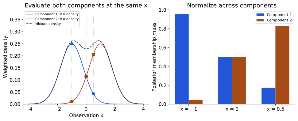
The specified model in Figure 18 has equal component masses, means \(-1\) and \(1\), and standard deviation \(0.8\). At \(x=0\), the weighted heights match, so responsibilities are \((0.5,0.5)\). At \(x=0.5\), the masses are approximately \((0.173,0.827)\). The bars are probabilities of components given an observation. This is a different normalization from t-SNE’s probabilities of other observations given an anchor: the normal curves play a related weighting role, but the outcomes being assigned probability have changed.

EM: replace hard counts with soft counts

How do we fit the mixture if component identities are not observed? Expectation–maximization (EM) alternates inference about those identities and parameter updates. Starting from valid parameters, its main operations are:

Step	Operation	Interpretation
E-step	Compute \(r_{ik}\) with the current mixture using Bayes’ rule.	Infer soft membership for each observation.
M-step: counts	\(N_k=\sum_i r_{ik}\); \(\pi_k\leftarrow N_k/n\).	Replace integer counts with effective counts.
M-step: means	\(m_k\leftarrow N_k^{-1}\sum_i r_{ik}x_i\).	Move each mean using weighted contributions.
M-step: covariances	\(\Sigma_k\leftarrow N_k^{-1}\sum_i r_{ik}(x_i-m_k)(x_i-m_k)^\top\).	Update spread about the newly updated mean.
Repeat	Recompute responsibilities, then parameters, until a declared stopping rule.	Fit a local solution to the mixture likelihood objective.

These formulas are for unconstrained full covariances and nonzero \(N_k\). Covariance constraints require corresponding updates; numerical implementations often add covariance regularization and handle very small component counts explicitly. Exact EM steps optimize a likelihood bound and cannot decrease observed-data log likelihood under their usual valid-update assumptions. They do not necessarily improve k-means inertia, which is a different objective. Unregularized mixtures can become singular as a component collapses onto an observation, so unconstrained likelihood maximization is not automatically well behaved.

To see the soft-count idea numerically, use observations \((-2,-1,1,2)\) with the same two-component model as above and keep its variance fixed at \(0.8^2\). An E-step followed by the mean/weight M-step gives effective counts \((2,2)\), masses \((0.5,0.5)\) and means approximately \((-1.454,1.454)\). Each point contributes to both components in proportion to its responsibility; a point does not need to be copied into a second hard group.

K-means and mixtures therefore share an alternating pattern, but their assumptions differ. With equal component masses and a common spherical covariance, the most probable component is the nearest mean. As that common variance tends to zero, non-tied responsibilities concentrate on the nearest component, connecting soft membership to hard assignment. A general fitted GMM also learns density and spread, so it should not be described as simply k-means with probability labels added.

What to carry forward. A group depends on a representation, a metric and an objective. K-means fits hard assignments and representative means; mixtures introduce a latent component and infer soft membership under a probability model. These constructions need evidence matched to their purpose, rather than a visually appealing partition alone.

Pause and interpret. Why can both corner partitions be stable even though their losses differ? Which changes the model: trying another initialization or scaling one feature? At the midpoint of two normal components, what assumptions gave responsibilities of one half each? Finally, can a Gaussian component be identified with a digit class without additional evidence?

TODO(instructor): review the clustering draft, exact Lloyd trace and mixture bridge. Full mixture-model/EM derivations remain optional, consistent with the syllabus; this section supplies the inference/update intuition rather than the full bound proof.

Autoencoders (AE): learning to reconstruct

PCA encodes an observation using a fixed linear basis and reconstructs it in the corresponding subspace. What if the variation we want to retain bends? An autoencoder (AE) replaces those linear operations with trainable functions:

\[ h=f_\psi(x)\in\mathbb R^d,\qquad \widehat x=g_\theta(h)\in\mathbb R^D. \]

Here code means the vector \(h\) of learned numerical features representing an image, not computer program code. The same encoder weights \(\psi\) are used for every image, but the resulting vector \(h=f_\psi(x)\) depends on the input image. The decoder uses shared weights \(\theta\) to reconstruct the image from \(h\). The original image supplies the reconstruction target; no digit-name labels are needed for training (Goodfellow et al. 2016, chap. 14).

Figure 19: Schematic of autoencoder training. The encoder maps an input image \(x\) to a numerical code \(h\), and the decoder produces its reconstruction \(\widehat x\). The original image supplies the reconstruction target. The mean squared error loss is backpropagated through both networks to update the encoder and decoder weights. The displayed code values and digit images are illustrative rather than measured outputs; the code dimension is a model choice.

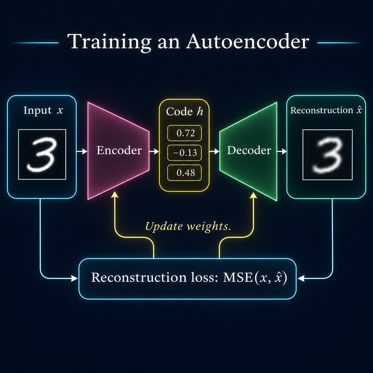
For continuous intensity images, a common objective is mean squared error over batch images and pixels:

\[ L_{\mathrm{AE}}=\frac1{BD}\sum_{i=1}^B\sum_{j=1}^D (x_{ij}-\widehat x_{ij})^2. \]

Here \(B\) is batch size, \(D\) input dimension and \(d\) code dimension. With observations as rows, shapes are \(X:(B,D)\), \(H:(B,d)\) and \(\widehat X:(B,D)\). Training backpropagates through the composition \(g_\theta(f_\psi(X))\). Encoding a new image uses a forward pass, rather than a new optimization of its code.

If a network can simply copy every input, reconstruction need not teach it a useful representation. An undercomplete bottleneck (\(d<D\)), architecture choices or other constraints force the model to prioritize information. A small bottleneck alone does not guarantee meaningful features: a flexible model can still memorize a finite dataset or preserve nuisance variation. Reconstruction checks on new data remain necessary.

Algorithm: train, then encode and reconstruct

Stage	Operation	What changes?
Specify	Choose the encoder, decoder, code dimension and reconstruction loss.	The model family and intended information constraint.
Forward	For a training batch, calculate \(H=f_\psi(X)\) and \(\widehat X=g_\theta(H)\).	Image-dependent codes and predictions.
Score	Compare \(\widehat X\) with the same batch \(X\).	A scalar training objective.
Update	Clear gradients, differentiate the loss through both networks, and take an optimizer step.	Shared encoder and decoder weights.
Check	Measure reconstruction on held-out observations using the fixed weights.	Evidence beyond fitting the training images.
Use	Encode a new image with \(f_\psi\); reconstruct its code with \(g_\theta\).	The image-dependent code and reconstruction; weights stay fixed.

What changes relative to PCA?

A centered linear encoder–decoder trained with squared error can, at an appropriate global optimum, reconstruct through the same principal subspace as PCA. Its internal code need not be PCA’s ordered orthonormal scores: an invertible change of latent coordinates can be absorbed by the decoder. Nonlinear activations allow a richer reconstruction function, but finite neural training need not find a better solution than exact PCA.

MNIST: train and inspect the AE

Our experiment uses 784 → 128 → d → 128 → 784, with ReLU hidden activations, a linear code, and a sigmoid reconstruction output. The sigmoid constrains predicted intensities to \([0,1]\). PCA reconstruction had no such constraint. Equal bottleneck size therefore does not make the methods identical in capacity, optimization, or output family.

We train \(d=2\) and \(d=16\) on the same 6,000 training images used for PCA and evaluate reconstruction on the same 1,000 validation images. Validation images are not used to update network weights. Both subsets come from MNIST’s official training partition; the official test set remains unused. Both runs use initialization seed 0, 20 epochs, Adam learning rate 0.001 and batches of 128. The settings and displayed image IDs were fixed before running; all declared runs are retained. This is a small CPU illustration, not a tuned benchmark or an evaluation on previously unseen writers.

Figure 20: Training-pass and held-out reconstruction errors for two autoencoder bottlenecks.

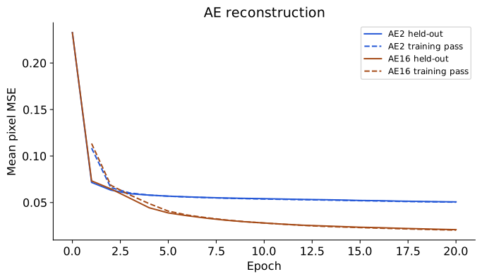
In Figure 20, the training curve averages losses encountered while the weights were changing within an epoch. The held-out curve uses the model at the epoch endpoint. Their difference is not a controlled estimate of a generalization gap at identical weights.

Figure 21: The same five held-out MNIST images reconstructed by the two autoencoders.

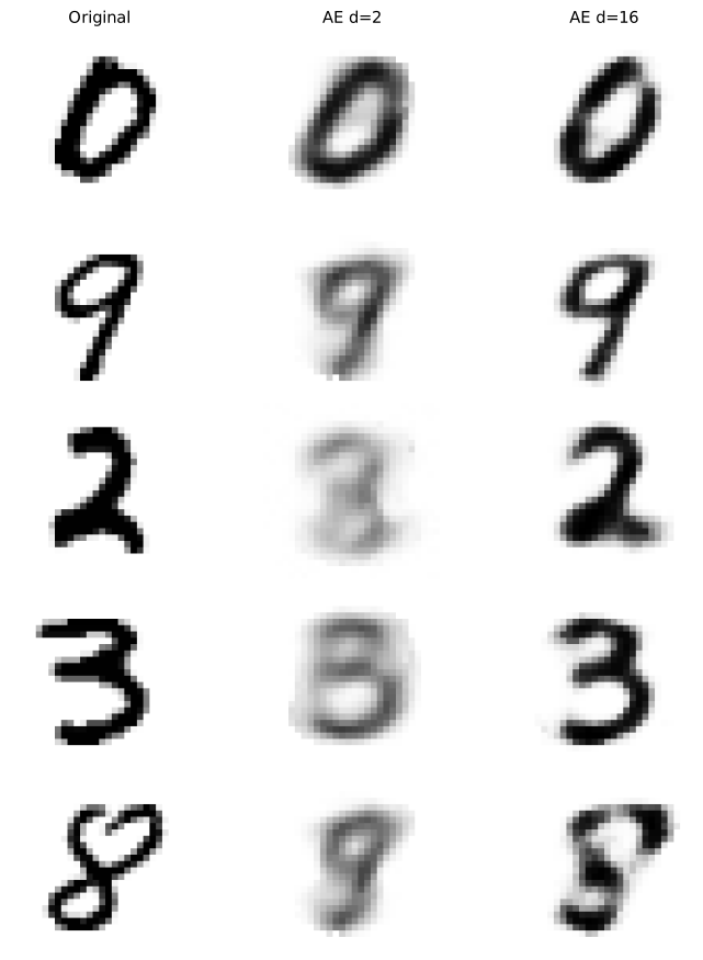
Each row in Figure 21 compares reconstructions of the same observation. Sixteen coordinates give this AE more room to retain detail than two. All panels use the fixed grayscale range \([0,1]\); the images retain their full 28×28 pixel resolution.

Does reconstruction give useful features?

An accurate reconstruction establishes recovery of pixel intensities under the chosen loss. Useful digit recognition is a different claim. To test it, freeze the encoder, encode training images, fit a declared classifier using training digit labels, choose classifier settings on validation data, and evaluate the frozen procedure on independent test data. This probe introduces supervised information at evaluation time, after representation learning.

The existing tutorial’s N05–N06 scenes implement reconstruction and frozen-probe comparisons on 8×8 optical digits. Those results do not establish probe performance for this new 28×28 experiment. The tutorial revision should reproduce the comparison on the chapter’s data contract; no recognition scores are inferred from the pictures here.

Optional connection: a denoising autoencoder

A denoising objective uses a corrupted input \(x^{\mathrm{corrupt}}\) but retains the clean observation \(x\) as its target. For Gaussian corruption, \(x^{\mathrm{corrupt}}=x+\eta\) with \(\eta\sim\mathcal N(0,s_n^2I)\). We use a superscript here to distinguish corruption from PCA’s centered observations.

Under population squared-error risk, the optimal prediction at a fixed corrupted input is

\[ \widehat x^*(x^{\mathrm{corrupt}}) =\mathbb E[x\mid x^{\mathrm{corrupt}}]. \]

To see why, expand the conditional expected squared error around the conditional mean. The cross term vanishes because \(x-\mathbb E[x\mid x^{\mathrm{corrupt}}]\) has conditional mean zero. What remains is an irreducible conditional variance plus the squared distance of the prediction from that mean. A finite neural model only approximates this optimum. With several plausible clean images, the conditional mean can lie between them and appear blurred.

This posterior is over a clean observation given its corrupted version. The VAE below instead infers an unobserved latent code given an observation. Denoising connects to score-based methods under additional assumptions, but a denoiser alone is not yet a complete specification of a generative sampling algorithm. We leave that extension outside the main chapter route.

The missing ingredient for generation

After AE training, we can encode an image and reconstruct it from that code. Where should a new code come from? A reconstruction objective does not specify a prior distribution or fit the density of encoded observations. Arbitrary code draws may visit regions poorly covered during training. Interpolation can sometimes work well, but reconstruction alone supplies no guarantee for every path or random draw.

This suggests specifying the generator explicitly: choose a distribution of codes and a distribution of observations conditional on a code. Learning and inference can then be derived from that model.

TODO(instructor): review the new AE experiment and short denoising extension. The held-out reconstructions are measured results; the downstream-recognition comparison remains tutorial work.

Variational autoencoders (VAE): loss and training

A variational autoencoder (VAE) learns an encoder and a decoder together. The encoder gives each input image a distribution of possible codes. The decoder reconstructs the image from a sampled code. The input image itself supplies the reconstruction target; no digit label or correct code is provided (Kingma and Welling 2014).

The explanation follows the training process: define the encoder and decoder, derive the loss, understand its two terms, and use them in one parameter update. The derivation appears once, in the main text. Code and inference-time generation follow as supplementary material.

Vectors and matrices are written in bold; individual coordinates and scalar quantities are not. The latent code is denoted by \(\mathbf{z}\). Distinguish three distributions over this code:

• Prior \(p(\mathbf{z})\): the chosen distribution of codes before observing a particular image. Here it is the fixed standard normal, \(\mathcal N(\mathbf{0},\mathbf{I})\), shared by all images.
• Posterior \(p_\theta(\mathbf{z}\mid \mathbf{x})\): the distribution of codes that could explain a particular observed image \(\mathbf{x}\) under the current decoder model. It depends on the image.
• Approximate posterior \(q_\psi(\mathbf{z}\mid \mathbf{x})\): the encoder’s computable approximation to that posterior. We use it because the exact posterior is generally difficult to calculate.

These distributions describe an image’s latent code, not uncertainty over the network weights. “Before” and “after” refer to observing the image, not to training epochs.

Training in one picture

Figure 22: Schematic representation of VAE training for a two-dimensional latent code (\(d=2\)); the formulation in the text applies to arbitrary \(d\). For each input image, the encoder defines an approximate posterior over latent codes, a code is sampled, and the decoder produces a reconstruction. Colored clouds denote image-specific code distributions, not digit classes; the yellow cloud denotes the fixed prior \(p(\mathbf{z})=\mathcal N(\mathbf{0},\mathbf{I})\) used for generation. In the illustration, \(\phi\) denotes the encoder weights \(\psi\), and \(\boldsymbol{\sigma}\) denotes standard deviation. Cloud orientations and reconstructed digits are illustrative rather than empirical; the implemented encoder uses diagonal covariance.

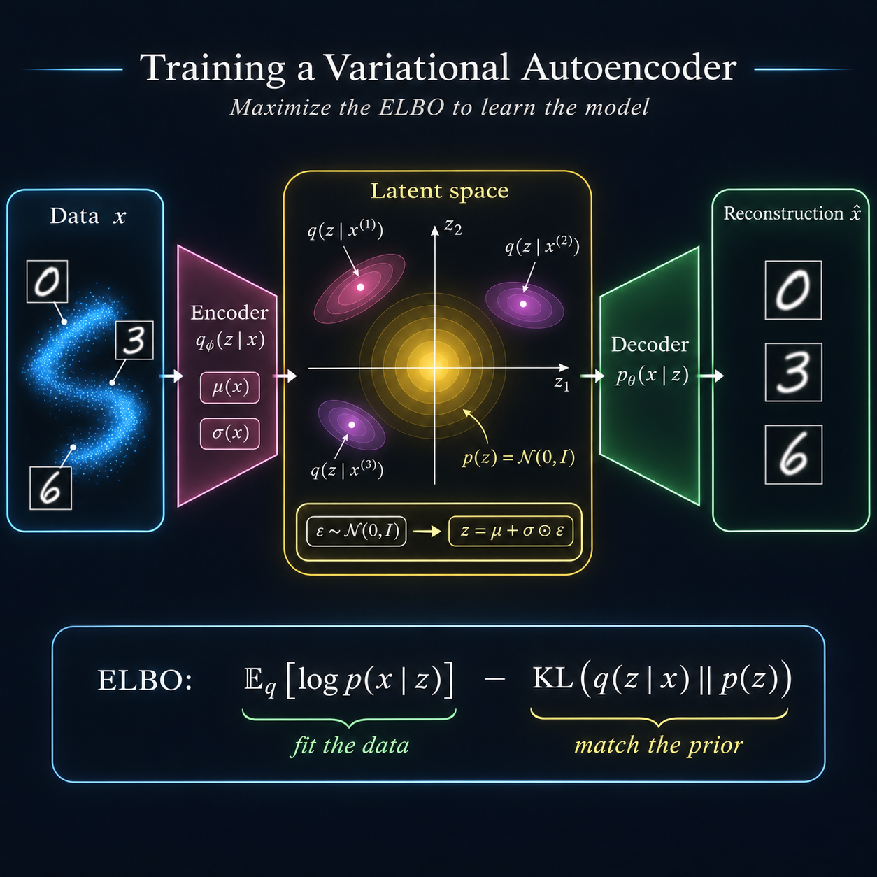
The loss has two jobs

A VAE minimizes reconstruction cost + prior KL cost. Reconstruction rewards codes that retain information about the input image. The prior KL compares that image’s approximate posterior from the encoder with the shared prior. The following derivation explains why these two terms belong together and how to calculate them.

What the two networks produce

Let \(d\) be the latent-code dimension. For each image \(\mathbf{x}\), the encoder produces two vectors of length \(d\):

\[ \boldsymbol{\mu}(\mathbf{x})\in\mathbb R^d,\qquad \log\boldsymbol{\sigma}(\mathbf{x})\in\mathbb R^d. \]

Each latent coordinate has one mean and one standard deviation, so the encoder produces \(2d\) scalar values in total. Here \(\sigma_k\) is the standard deviation of coordinate \(k\), and \(\sigma_k^2\) is its variance. For a batch of \(B\) images, each output has shape \((B,d)\).

Exponentiating the second vector coordinatewise gives positive standard deviations, \(\boldsymbol{\sigma}=\exp(\log\boldsymbol{\sigma})\), and squaring gives variances, \(\boldsymbol{\sigma}^2=\exp(2\log\boldsymbol{\sigma})\). The covariance matrix places these variances on its diagonal. These vectors define the approximate posterior

\[ q_\psi(\mathbf{z}\mid \mathbf{x})=\mathcal N\!\left(\mathbf{z};\boldsymbol{\mu}(\mathbf{x}),\operatorname{diag}(\boldsymbol{\sigma}(\mathbf{x})^2)\right). \]

Here \(\psi\) denotes the encoder weights. The weights are shared across images, while \(\boldsymbol{\mu}(\mathbf{x})\) and \(\boldsymbol{\sigma}(\mathbf{x})\) depend on the image. The prior remains the same for all images.

The decoder network, with weights \(\theta\), takes a latent code \(\mathbf{z}\), not an image, as input. Its output \(g_\theta(\mathbf{z})\in\mathbb R^D\) is a vector of \(D\) predicted pixel means: a reconstructed mean image. Here \(g_\theta\) names the neural-network function.

To turn that prediction into a probability model, we specify how images can vary around it. For continuous pixels, we use a Gaussian image model with a fixed pixel standard deviation \(s_x>0\), shared across pixels:

\[ p_\theta(\mathbf{x}\mid \mathbf{z})=\mathcal N\!\left(\mathbf{x};g_\theta(\mathbf{z}),s_x^2\mathbf{I}\right). \]

Thus \(g_\theta(\mathbf{z})\) and \(p_\theta(\mathbf{x}\mid\mathbf{z})\) are different objects: the first is a predicted image vector; the second is a scalar probability density evaluated at an image \(\mathbf{x}\), with that vector as its Gaussian mean. The marginal density \(p_\theta(\mathbf{x})\) averages over possible codes, as derived next.

The encoder’s \(\boldsymbol{\sigma}\) describes spread in code space; \(s_x\) describes spread around the decoder’s image prediction. They are different quantities.

Deriving and understanding the VAE loss

Start with the probability of an observed image

We want the decoder model to explain the training images. For one image \(\mathbf{x}\), its model density averages over the unobserved code:

\[ p_\theta(\mathbf{x})=\int p_\theta(\mathbf{x}\mid \mathbf{z})p(\mathbf{z})\,d\mathbf{z}. \]

A code contributes when it is plausible under the prior and the decoder assigns high density to \(\mathbf{x}\) from that code. Learning by maximum likelihood would increase \(\log p_\theta(\mathbf{x})\), summed over the training images. The obstacle is the integral: with a nonlinear neural decoder, we generally cannot evaluate it exactly.

The encoder \(q_\psi(\mathbf{z}\mid \mathbf{x})\) gives us a distribution from which we can sample candidate codes for this particular image. It approximates the model’s exact posterior \(p_\theta(\mathbf{z}\mid \mathbf{x})\). We do not have posterior distributions as training targets. Instead, we derive a computable objective that trains both networks from the observed images.

Derive one computable lower bound

Fix an observed image \(\mathbf{x}\). KL divergence compares two distributions over the latent code, rather than their density values at a single code. For the encoder distribution and the exact posterior, its definition gives:

\[ \begin{aligned} D_{\mathrm{KL}}(q_\psi(\mathbf{z}\mid\mathbf{x})\|p_\theta(\mathbf{z}\mid \mathbf{x}))\\ &=\mathbb E_{q_\psi(\mathbf{z}\mid\mathbf{x})}[\log q_\psi(\mathbf{z}\mid\mathbf{x})-\log p_\theta(\mathbf{z}\mid \mathbf{x})]. \end{aligned} \]

This equality is the exact definition of KL divergence, not an approximation; the expectation averages over codes drawn from the encoder for this fixed image.

Bayes’ rule gives \(\log p_\theta(\mathbf{z}\mid \mathbf{x})=\log p_\theta(\mathbf{x}\mid \mathbf{z})+\log p(\mathbf{z})-\log p_\theta(\mathbf{x})\). Substituting and grouping terms yields

\[ \begin{aligned} D_{\mathrm{KL}}(q_\psi(\mathbf{z}\mid\mathbf{x})\|p_\theta(\mathbf{z}\mid \mathbf{x})) &=\mathbb E_{q_\psi(\mathbf{z}\mid\mathbf{x})}[\log q_\psi(\mathbf{z}\mid\mathbf{x})-\log p(\mathbf{z})]\\ &\quad-\mathbb E_{q_\psi(\mathbf{z}\mid\mathbf{x})}[\log p_\theta(\mathbf{x}\mid \mathbf{z})]+\log p_\theta(\mathbf{x}). \end{aligned} \]

The first expectation is \(D_{\mathrm{KL}}(q_\psi(\mathbf{z}\mid\mathbf{x})\|p(\mathbf{z}))\), the divergence to the prior. Rearranging gives

\[ \begin{aligned} \log p_\theta(\mathbf{x}) &=\underbrace{\mathbb E_{q_\psi(\mathbf{z}\mid\mathbf{x})}[\log p_\theta(\mathbf{x}\mid \mathbf{z})] -D_{\mathrm{KL}}(q_\psi(\mathbf{z}\mid\mathbf{x})\|p(\mathbf{z}))}_{\mathcal E(\mathbf{x})\;\text{(ELBO)}}\\ &\quad+D_{\mathrm{KL}}(q_\psi(\mathbf{z}\mid\mathbf{x})\|p_\theta(\mathbf{z}\mid \mathbf{x})). \end{aligned} \]

KL divergence is nonnegative, so \(\mathcal E(\mathbf{x})\leq\log p_\theta(\mathbf{x})\). This is the evidence lower bound (ELBO). We can calculate or estimate its two terms without evaluating the difficult evidence integral or exact posterior. Maximizing this bound is the VAE training objective (Kingma and Welling 2014).

Optimizers usually minimize a loss, so change its sign:

\[ \boxed{\mathcal L(\mathbf{x})= \underbrace{\mathbb E_{q_\psi(\mathbf{z}\mid \mathbf{x})}[-\log p_\theta(\mathbf{x}\mid \mathbf{z})]}_{\text{reconstruction cost}} + \underbrace{D_{\mathrm{KL}}(q_\psi(\mathbf{z}\mid \mathbf{x})\|p(\mathbf{z}))}_{\text{prior KL cost}}.} \]

There are two KL divergences in the derivation, but only the prior KL is calculated in the loss. The KL to the exact posterior is the gap between the bound and the log evidence. It explains the approximation; it is not an extra penalty to calculate. Both encoder and decoder are optimized through the same loss.

Reconstruction cost: make the sampled code explain the input

Fix the original image \(\mathbf{x}\) and one code \(\mathbf{z}\) sampled from its encoder distribution. The decoder returns one Gaussian mean per pixel in \(g_\theta(\mathbf{z})\); the model fixes each pixel variance at \(s_x^2\). In this Gaussian image model,

\[ p_\theta(\mathbf{x}\mid \mathbf{z})=(2\pi s_x^2)^{-D/2} \exp\!\left[-\frac{\|\mathbf{x}-g_\theta(\mathbf{z})\|^2}{2s_x^2}\right], \]

where \(D\) is the number of pixels. Evaluate each pixel’s Gaussian density at its observed value in \(\mathbf{x}\). Because pixels are conditionally independent given \(\mathbf{z}\), the whole-image density is the product over pixels. Taking the negative logarithm turns that product into a sum over pixels, giving one scalar cost for the image.

Keep \(\mathbf{x}\) fixed and draw a second code from the encoder: its decoded means give a new whole-image cost. The expectation in \(\mathcal L(\mathbf{x})\) averages these costs over latent codes; training estimates it with one draw per image. For a single draw, the cost is

\[ \operatorname{NLL}(\mathbf{x},\mathbf{z}) =\frac{\|\mathbf{x}-g_\theta(\mathbf{z})\|^2}{2s_x^2} +\frac D2\log(2\pi s_x^2). \]

The squared residual compares the reconstruction with the same input image, pixel by pixel. A missing stroke increases this term; recovering it decreases the term. Since \(s_x\) is fixed, the second term is a constant with respect to the network weights. The reconstruction gradient therefore comes from the scaled squared error. The likelihood choice determines this formula; a Bernoulli pixel model would give binary cross-entropy instead.

Through the sampled code, reconstruction gradients tell the encoder which proposals help the decoder, while also updating the decoder itself.

A four-pixel example. Consider a \(2\times2\) grayscale image, flattened row by row as \(\mathbf{x}=(0.7,0.4,0.1,0.9)\). The image has \(D=4\) pixel values; we choose a code with only \(d=2\) latent coordinates. The following encoder and decoder outputs are illustrative, not measured training results.

1. Encode and sample. Suppose the encoder gives \(\boldsymbol{\mu}=(2,-1)\) and \(\boldsymbol{\sigma}=(0.5,0.2)\). With standard-normal noise \(\boldsymbol{\epsilon}=(1,-0.5)\), the sampled code is \(\mathbf{z}=\boldsymbol{\mu}+\boldsymbol{\sigma}\odot\boldsymbol{\epsilon}=(2.5,-1.1)\).

2. Decode. Suppose \(g_\theta(\mathbf{z})=(0.8,0.2,0.2,0.8)\) and choose \(s_x=0.25\). The decoder gives four pixel means from the two-coordinate code. Each pixel has its own Gaussian mean and the same variance \(0.25^2\).

3. Score the original image. Evaluate the four Gaussian densities at the observed values \(0.7\), \(0.4\), \(0.1\) and \(0.9\), obtaining \(d_1,d_2,d_3,d_4\). Their product is the whole-image density. Its negative logarithm is

   \[ -\sum_{j=1}^{4}\log d_j =0.08+0.32+0.08+0.08+C=0.56+C, \]

   where \(C=2\log(2\pi s_x^2)\) is fixed. This is one scalar cost for the whole image at this code. Another code for the same image can give another cost; averaging over codes gives the reconstruction expectation. This training step uses one draw.

Prior KL cost: regulate the center and spread of each code distribution

Our encoder is a diagonal Gaussian with coordinate means \(\mu_k\) and variances \(\sigma_k^2=\exp(2\log\sigma_k)\). The prior has zero means and unit variances. For one latent coordinate, the log-density ratio is

\[ \log\frac{q(z_k\mid \mathbf{x})}{p(z_k)} =-\log\sigma_k-\frac{(z_k-\mu_k)^2}{2\sigma_k^2}+\frac{z_k^2}{2}. \]

Under \(q\), \(\mathbb E[(z_k-\mu_k)^2]=\sigma_k^2\) and \(\mathbb E[z_k^2]=\mu_k^2+\sigma_k^2\). Taking the expectation and summing independent coordinates gives

\[ \begin{aligned} D_{\mathrm{KL}}(q_\psi(\mathbf{z}\mid \mathbf{x})\|p(\mathbf{z})) &=\frac12\sum_{k=1}^d [\mu_k^2+\sigma_k^2-1-\log\sigma_k^2]\\ &=\frac12\sum_{k=1}^d [\mu_k^2+\exp(2\log\sigma_k)-1-2\log\sigma_k]. \end{aligned} \]

The expression separates two effects:

• \(\mu_k^2\) charges for moving the center away from zero. A distant image-specific center costs more.
• \(\sigma_k^2-1-\log\sigma_k^2\) charges for changing the spread away from one. It increases for both very narrow and very wide distributions. Its minimum is at \(\sigma_k^2=1\), not zero.

Unlike reconstruction, this term needs no sampled code: it is calculated directly from the encoder’s predicted means and log standard deviations.

Complete the four-pixel example: add KL and update. Applying the formula above to \(\boldsymbol{\mu}=(2,-1)\) and \(\boldsymbol{\sigma}=(0.5,0.2)\) gives a prior KL of approximately \(3.95\). Omitting the fixed constant for optimization gives a one-draw loss of \(0.56+3.95=4.51\). Keeping \(C\) gives the actual NLL and negative-ELBO estimate; omitting it leaves the gradients unchanged. Backpropagation carries reconstruction gradients into both networks and prior-KL gradients into the encoder.

Why neither term is sufficient alone

For an image of a 3, reconstruction rewards a code that lets the decoder recover its strokes. With reconstruction alone, there is no explicit penalty for assigning images remote, extremely narrow code distributions. The prior KL opposes those departures from the shared normal reference.

With KL alone, every image could receive the same standard-normal distribution and pay zero cost. Such codes carry no information about which image entered the encoder. Reconstruction supplies the opposing pressure to retain useful image information. The combined objective balances these demands; it does not require all image-specific distributions to become identical.

A low total loss must therefore be interpreted with its two components. A low KL does not by itself establish good reconstruction, and a low reconstruction error does not by itself establish a useful shared code distribution.

Sampling a code without blocking gradients

The sampled code must still let us train the encoder. Draw standard-normal noise, then shift and scale it using the encoder outputs:

\[ \begin{aligned} \boldsymbol{\epsilon}&\sim\mathcal N(\mathbf{0},\mathbf{I}_d),\qquad \boldsymbol{\sigma}=\exp(\log\boldsymbol{\sigma}),\\ \mathbf{z}&=\boldsymbol{\mu}+\boldsymbol{\sigma}\odot\boldsymbol{\epsilon}. \end{aligned} \]

The chain rule now carries reconstruction gradients through the decoder, through \(\mathbf{z}\), and into both encoder heads. Hold the drawn noise fixed while differentiating that forward pass; draw fresh noise on later training passes. Other gradient estimators exist, but this pathwise construction is the one used here.

Algorithm: one training step

Step	What happens
1. Encode	Give an image \(\mathbf{x}\) to the encoder. It predicts a code center \(\boldsymbol{\mu}\) and standard deviations \(\boldsymbol{\sigma}\).
2. Sample	Draw fresh noise \(\boldsymbol{\epsilon}\sim\mathcal N(\mathbf{0},\mathbf{I})\) and form \(\mathbf{z}=\boldsymbol{\mu}+\boldsymbol{\sigma}\odot\boldsymbol{\epsilon}\). The symbol \(\odot\) means coordinatewise multiplication.
3. Reconstruct	Feed \(\mathbf{z}\) to the decoder and compare its predicted image with the original \(\mathbf{x}\).
4. Score	Add the reconstruction cost and the prior KL cost for this image. Average these sums across the batch.
5. Update	Backpropagate the combined loss and update both encoder and decoder weights. Repeat with another batch.

Each update changes the shared encoder and decoder weights; it does not optimize a separately stored code for each training image.

For a batch of \(B\) images, one code draw per image gives the training estimate

\[ \widehat{\mathcal L}_{\rm batch} =\frac1B\sum_{i=1}^B \left[\operatorname{NLL}(\mathbf{x}_i,\mathbf{z}_i) +D_{\mathrm{KL}}(q_\psi(\mathbf{z}\mid \mathbf{x}_i)\|p(\mathbf{z}))\right]. \]

Pixel losses and latent-coordinate KL contributions are summed within each image, then the combined costs are averaged across images. This reduction keeps the formulas above consistent with the optimizer step. Changing only one reduction would change the balance between reconstruction and KL.

Training a VAE on MNIST: reconstructions and code distributions

The VAE uses 784 → 128 → (mean, log standard deviation), two-dimensional latent codes, and 2 → 128 → 784 decoding with a sigmoid mean output. For this experiment, the fixed pixel standard deviation is \(s_x=0.25\). Training uses the same 6,000-training/1,000-validation image split, 20 epochs, Adam 0.001, batches of 128 and initialization seed 0 as the AE illustrations. The held-out NLL averages four fixed posterior-noise draws per image; training uses fresh noise. These are new runs, not recycled Week 07 or optical-digit metrics.

Figure 23: Training-pass and held-out values of the VAE’s two loss terms.

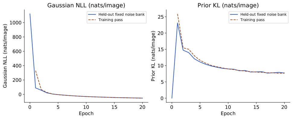
In Figure 23, NLL and KL measure different pressures and should be read separately. The first encourages codes that let the decoder explain each image. The second penalizes departures from the prior, including the information those image-specific codes carry. KL’s minimum occurs at zero mean and unit latent variance, not zero variance.

The reconstructions below decode the encoder’s mean code, a deterministic display that generally differs from averaging decoded posterior draws.

Figure 24: Original images and their mean-code reconstructions under the standard VAE.

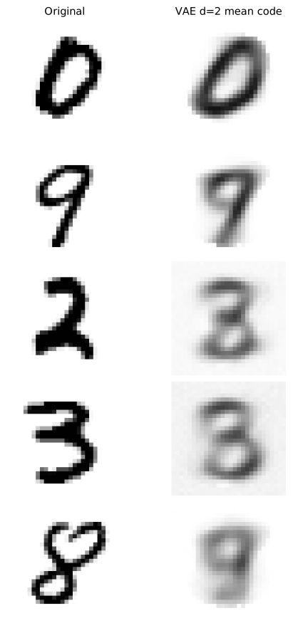
The same observations appear in Figure 21 and Figure 24. Compare what detail survives, while remembering that the AE and VAE optimize different objectives. A less detailed VAE reconstruction does not by itself establish worse prior generation, and a sharper AE reconstruction does not supply a sampling law.

Figure 25: AE codes are points; VAE inference includes both a center and an image-specific spread.

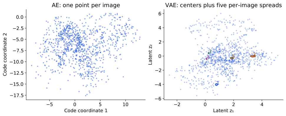
Each ellipse in Figure 25 has coordinate semiaxes of one standard deviation. It is a geometric spread illustration, not a stated 95% region. The points alone omit those spreads. The aggregate distribution of codes across images is a mixture of their approximate posteriors, not simply the scatter of means; the KL objective does not guarantee that aggregate is exactly standard normal or that its axes describe named semantic factors.

VAE diagnostics: KL weighting and posterior collapse

Changing the prior-KL coefficient gives

\[ L_\beta=\frac1B\sum_i[\widehat{\operatorname{NLL}}_i+ \beta D_{\mathrm{KL}}(q_\psi(\mathbf{z}\mid \mathbf{x}_i)\|p(\mathbf{z}))]. \]

Only \(\beta=1\) is the standard negative-ELBO objective for the stated model. For the diagnostic comparison, we train \(\beta=4\) from the same initial parameters with the same batch order and noise streams as \(\beta=1\). Compare unweighted NLL and KL separately; differently weighted totals are not a likelihood ranking.

The table compares the two VAE runs alongside the AEs introduced earlier. Their losses retain their stated units and reductions.

Model	Held-out reconstruction	Prior KL (nats/image)
AE2	MSE 0.0507	—
AE16	MSE 0.0209	—
VAE1	Gaussian NLL -52.51 nats/image	7.74
VAE4	Gaussian NLL -48.04 nats/image	4.26

AE2 and AE16 denote the two deterministic bottlenecks. VAE1 uses the standard coefficient \(\beta=1\); VAE4 uses \(\beta=4\) in the paired experiment just described. AE reconstruction entries are MSE; VAE reconstruction entries are Gaussian NLL, so the table is not a common-score ranking.

Posterior collapse means the inferred code conveys little useful image-specific information and the decoder largely ignores it. Low KL is a clue, not a sufficient diagnosis on its own. Test the decoder’s dependence on the code by replacing each image’s mean code with zero or with another image’s code, measuring reconstruction against the same originals.

KL weight	Mean-code MSE	Zero-code MSE	Shuffled-code MSE
1	0.0499	0.0879	0.0875
4	0.0500	0.0785	0.0867

In this paired run, \(\beta=4\) reduces prior KL and increases unweighted reconstruction NLL. Both models reconstruct less accurately after their codes are replaced: these checks show code dependence, rather than complete posterior collapse.

These are deterministic MSE diagnostics on the same held-out observations, not ELBO estimates or causal isolation of every training effect. A larger error after intervention shows that those codes matter to reconstruction in this experiment. Per-coordinate KL, variation of the encoder means and the generated images provide additional views. Stronger KL weighting does not guarantee collapse, better samples, or disentanglement.

Blurry mean reconstructions can involve the observation model, bottleneck capacity, posterior approximation and optimization as well as regularization. A Gaussian pixel model can favor averaged predictions when several observations remain plausible. Our small network and short training budget also limit what it can learn. We should report those limits rather than attribute all blur to a single term.

Supplement: gradients and implementation

AE mean-pixel MSE and VAE NLL have different reductions and scales. Dividing only NLL by \(D\) while retaining the same KL would change their relative influence. The Gaussian constant is fixed for gradient optimization here, but keep it when reporting likelihood-based numbers. Gaussian densities can exceed one, so NLL can be negative. A negative density NLL does not mean negative squared error. Learning \(s_x\) would require a different model and retaining its log-variance contribution.

Scaling uses standard deviation, not variance. For one coordinate and one fixed noise draw,

\[ \frac{\partial z_k}{\partial\mu_k}=1,\qquad \frac{\partial z_k}{\partial(\log\sigma_k)}=\sigma_k\epsilon_k. \]

Figure 26: The same noise points are shifted and stretched to show how encoder outputs determine sampled codes.

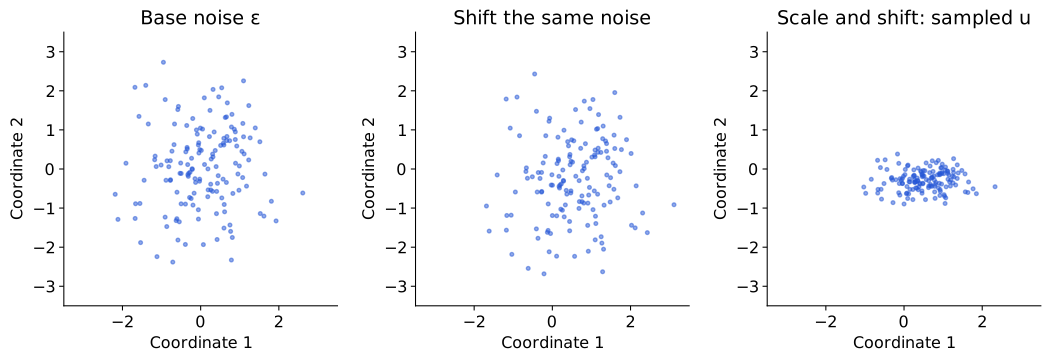
In Figure 26, the points move continuously when the mean or spread changes. Fixing the noise here isolates those effects. It does not remove stochasticity from training or turn a set of image-code means into the complete posterior distribution.

This short function spells out the same step for the existing Gaussian VAE and optimizer. Its encode method stores log variances, so the code first divides them by two to obtain \(\log\boldsymbol{\sigma}\). This conversion preserves the same distribution and loss:

import math
import torch

def gaussian_vae_step(model, optimizer, x, observation_sd=0.25):
    model.train()
    optimizer.zero_grad()
    mu, log_variance = model.encode(x)         # (B, d), (B, d)
    log_sigma = 0.5 * log_variance              # convert to log standard deviation
    sigma = log_sigma.exp()
    epsilon = torch.randn_like(mu)
    z = mu + sigma * epsilon
    mean = model.decoder(z)                    # (B, D)
    nll = ((mean - x) ** 2).sum(1) / (2 * observation_sd**2)
    nll = nll + x.shape[1] / 2 * math.log(2 * math.pi * observation_sd**2)
    kl = 0.5 * (mu.square() + sigma.square() - 1 - 2 * log_sigma).sum(1)
    loss = (nll + kl).mean()
    loss.backward()
    optimizer.step()
    return nll.detach().mean(), kl.detach().mean()

The figure generator checks the analytic KL and Gaussian NLL against PyTorch distributions. It also executes a complete optimizer step from fresh parameters, asserting nonzero finite gradients in encoder, both heads and decoder, and changes in their parameters. These checks establish the training mechanism, not successful generalization. Evaluating a trained model uses fixed weights; eval() does not itself switch off explicitly written random latent sampling. We choose mean-code reconstruction or a declared noise bank explicitly.

NoteConnection to Week 07: why BCE there and squared residuals here?

The reconstruction term follows the observation model, not the code prior. Week 07 thresholds pixels to zero or one and uses a Bernoulli observation model, which gives binary cross-entropy (BCE). Here we keep continuous intensities and use a Gaussian observation model, which gives the scaled squared residuals derived above. This comparison matters when reusing the tutorial code: changing the observations requires checking the likelihood and its loss.

Example	Observation model	Decoder output	Reconstruction term
Week 07 chapter/tutorial	Bernoulli pixels for thresholded 28×28 MNIST	Pixel logits, transformed to probabilities	Summed pixel BCE
Existing Week 10 tutorial	Gaussian pixels for continuous 8×8 optical digits	Mean image; fixed \(s_x=0.25\)	Gaussian negative log likelihood
This chapter’s new experiment	Gaussian pixels for continuous 28×28 MNIST	Mean image; fixed \(s_x=0.25\)	Same Gaussian formula, with \(D=784\)

The latent-variable construction and inference procedure are shared, but the pixel likelihood determines the reconstruction term. See Week 07’s likelihood derivation for the Bernoulli case.

Figure 27: A VAE’s training path includes image-specific code distributions and a shared gradient update of both networks.

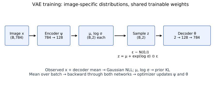
In Figure 27, the prior stays fixed, while encoder and decoder weights learn. For a fixed image, changing encoder weights changes its predicted mean and spread. Across epochs the decoder changes too, so the exact posterior being approximated also changes. Training is not simply adjusting each image’s Gaussian until it equals the prior.

Optional: generation and interpolation after training

With the trained weights fixed, draw a code from the prior and pass it through the decoder. There is no input image, encoder pass, reconstruction target, or weight update. This is a use of the trained model, separate from the training loop above.

Figure 28: Generation uses a trained decoder and a fresh prior code.

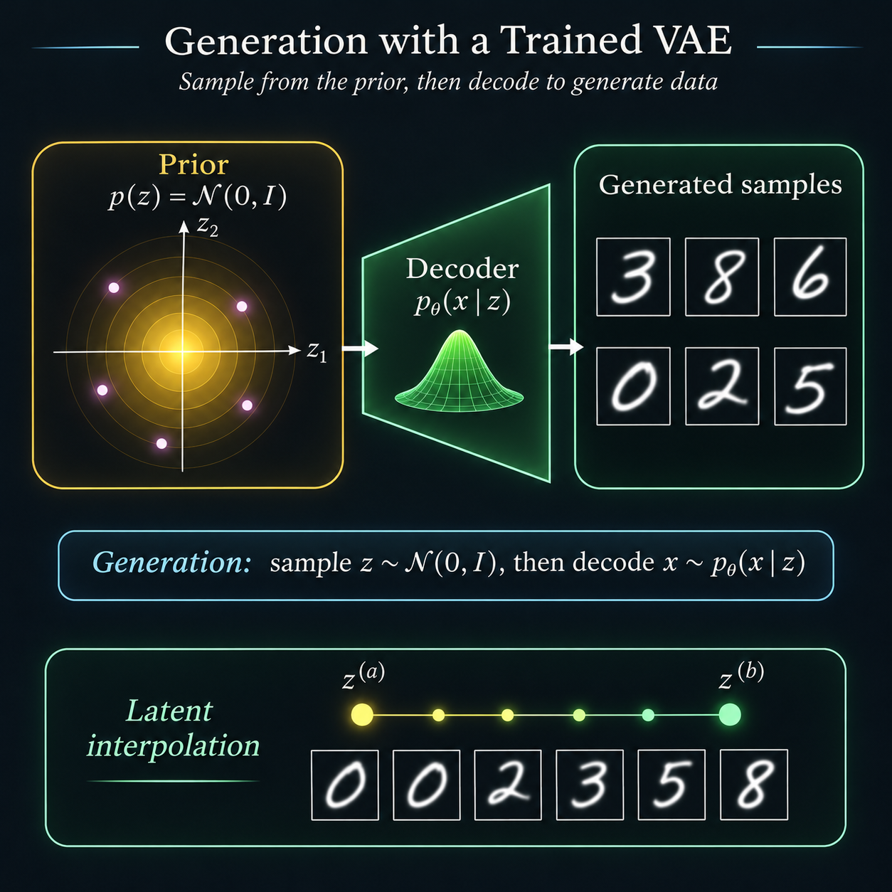
Its clean digit samples and interpolation sequence are schematic, not measured outputs or a guaranteed progression between digit classes. The lower panel chooses a path between codes; it is not random prior sampling. Measured decoder outputs are shown below.

Reconstruction, generation, and interpolation are separate operations

Operation	Algorithm with fixed weights	Output to label
Reconstruct	Given \(\mathbf{x}\), encode \(q_\psi(\mathbf{z}\mid \mathbf{x})\); use its mean or draw a code; decode.	Mean-code reconstruction or posterior-draw reconstruction
Generate	Draw a fresh \(\mathbf{z}\sim p(\mathbf{z})\); decode its observation parameters; optionally draw \(\mathbf{x}\sim p_\theta(\mathbf{x}\mid \mathbf{z})\).	Decoder mean or actual observation draw
Interpolate	Choose two codes and evaluate \((1-\alpha)\mathbf{z}^{(a)}+\alpha \mathbf{z}^{(b)}\) for specified \(\alpha\).	Chosen latent path, usually displayed as decoded means

Generation does not require an input image or the encoder. Reconstruction does. Interpolation fixes endpoints and a path; it is not a random draw from the prior.

Figure 29: Fresh prior codes produce decoder mean images and, separately, noisy observation draws from the stated Gaussian model.

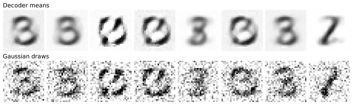
Figure 29 uses generation seed 77 and all eight prespecified prior codes. The observation draws can leave \([0,1]\) because the Gaussian model has real support. Display saturation clips only the plotted grayscale values; training and likelihood calculations use the unmodified values. The noise is a consequence of the observation model, not an extra decoder failure.

Figure 30: A chosen grid shows how the trained decoder mean varies with two latent coordinates.

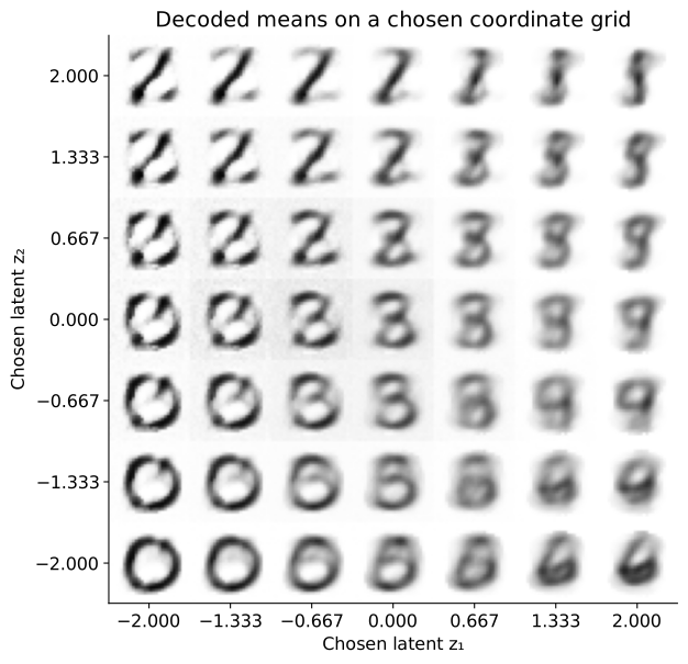
The atlas in Figure 30 evaluates a uniform coordinate grid. Uniform grid spacing is not probability-weighted prior sampling. It shows the decoder’s response at stated inputs, including regions where generated means may be poor. Neither the grid nor a smooth-looking interpolation proves that the model matches the data distribution.

Figure 31: A chosen line between the first two held-out posterior mean codes is decoded at eight positions.

In Figure 31, even the endpoints are reconstructions. A continuous neural decoder can change its outputs smoothly along this path; perceptual plausibility and semantic meaning require separate inspection. An ordinary AE may also interpolate well on some paths. The VAE’s advantage here is the specified sampling model and variational training objective, not a universal guarantee about every latent location.

TODO(instructor): review the VAE loss derivation, training explanation, and empirical figures. The supplied overview artwork is conceptual; the training curves and image outputs here come from the documented experiment. Broader conditional-VAE and diffusion extensions are outside this core route.

What did we learn without labels?

We began with four questions about observations without supplied task labels. They now have concrete methods and different kinds of evidence. The absence of digit labels during fitting did not remove our choices: feature units, distance, model family, bottleneck, likelihood and training budget all specified what structure to favor.

Opening question	What the chapter has actually demonstrated	What still needs checking or belongs in the tutorial
Can we compress?	PCA’s variance–error identity; held-out MNIST reconstruction; learned AE/VAE reconstructions under declared objectives.	Reproduce the same split, vary code dimension and budget, and compare like-for-like errors. Reconstruction alone does not establish recognition.
Can we group?	Exact k-means objective steps; effects of metric/start; curved-group failure; probabilistic mixture responsibilities.	Audit stability across starts and data perturbations. External label agreement needs a separately declared protocol.
Can we map?	PCA and t-SNE maps of the same observations; t-SNE neighborhood retention and trustworthiness across declared settings.	Inspect ambiguous images and stable neighbor IDs. A map does not establish a class count, density or globally calibrated distances.
Can we generate?	A specified VAE sampling law, a checked training step, trained prior decoder means and actual Gaussian observation draws.	Evaluate diversity and failure cases across additional runs. The displayed sample grid is not a quantitative proof of distributional fidelity.

One method, one objective, one interpretation

Method	Fitted output or representation	Main objective	New-observation operation
PCA	Linear coordinates and basis	Retained variance / squared reconstruction	Apply saved mean and basis
t-SNE	Coordinates for the fitted observations	Pair-affinity KL	Standard implementation here has no fixed arbitrary-input transform
K-means	Centers and hard groups	Squared distances to centers	Assign to saved nearest center
GMM	Component parameters and responsibilities	Mixture likelihood	Evaluate density and posterior component membership
AE	Deterministic encoder and decoder	Reconstruction loss	Encode and reconstruct with fixed networks
VAE	Generator plus approximate latent inference	ELBO for a declared likelihood	Infer a code for an image; independently generate from the prior

The VAE adds a probabilistic model, not just noise to an AE. Its posterior asks which hidden codes could explain an observed image; its prior supplies codes before any image is observed. The encoder approximates the former, while generation starts from the latter. Training joins inference and generation through a tractable bound on model evidence.

What the tutorial should establish next

The archived previous Week 10 tutorial contains PCA/AE reconstruction, a frozen recognition probe, clustering diagnostics, t-SNE audits and VAE training on 8×8 optical digits. It is an earlier draft and has not yet been revised to this chapter’s 28×28 MNIST experiments. Its numerical results must not be relabeled as results of this chapter’s models.

The active Week 10 tutorial is a classroom draft with challenges on denoising, retrieval and anomaly detection, plus optional mapping and generation activities. It uses offline 8×8 digits.

The tutorial revision should make the chapter’s questions executable in this order:

1. Lock the observations, preprocessing, training/validation/test roles and the question being tested before comparing models.
2. Reproduce compression and mapping; inspect both errors and individual data examples rather than choosing the prettiest map.
3. Fit reconstruction-based representations without labels, then explicitly introduce labels for a frozen downstream probe. Fit probe preprocessing on training codes, select on validation data and evaluate the frozen pipeline on test data.
4. Trace a VAE forward pass, verify NLL/KL reductions and gradients, then train and compare reconstruction, prior generation and code interventions as distinct checks.
5. Return to the opening evidence table and write a claim supported by each experiment, including a limitation and any use of labels.

That last step matters: no single score verifies “understanding.” A method can compress well yet lose a discriminative feature, produce a clear map while distorting global distances, or reconstruct well while generating poorly from its prior. The appropriate test follows the question.

Questions and exercises (optional)

1. For an AE with \(X:(B,784)\) and code dimension 16, state the encoder/decoder output shapes and the axis reductions in mean pixel MSE. Which quantities are shared parameters and which belong to an image?
2. A VAE has a normal code prior. Does that determine whether its reconstruction term is BCE or squared error? State what additional model choice is needed.
3. Explain the difference between \(p_\theta(\mathbf{z}\mid \mathbf{x})\) and \(q_\psi(\mathbf{z}\mid \mathbf{x})\). Which is the Bayesian inference target? What is learned without exact posterior labels?
4. Identify the two KL comparisons in the ELBO identity. Which one is calculated in our training loss? Must both vanish if the approximate posterior is exact?
5. Replace a pixel sum by a pixel mean without changing prior KL. What happens to the relative weighting when \(D=784\)? How would you preserve the original objective up to a common scale?
6. In reparameterization, explain what changes when log variance increases and why its exponential is divided by two before scaling the noise. Which quantities receive gradients?
7. Design a comparison that distinguishes accurate reconstruction from useful digit recognition. Specify where labels enter and how you will keep test data out of model selection.
8. Explain why decoded means, observation draws and interpolation grids are three different kinds of output. What evidence would you collect before claiming good generative modeling?

TODO(instructor): review the new AE/VAE sections, closing evidence audit and optional exercises. Revise the tutorial and slides after accepting the textbook narrative; the current tutorial link is a companion draft, not a claim that all planned revision checks have been completed.

References

Ba, Jimmy Lei, Jamie Ryan Kiros, and Geoffrey E. Hinton. 2016. “Layer Normalization.” arXiv Preprint arXiv:1607.06450. https://arxiv.org/abs/1607.06450.

Baydin, Atilim Gunes, Barak A. Pearlmutter, Alexey Andreyevich Radul, and Jeffrey Mark Siskind. 2018. “Automatic Differentiation in Machine Learning: A Survey.” Journal of Machine Learning Research 18 (153): 1–43. https://www.jmlr.org/papers/v18/17-468.html.

Bishop, Christopher M. 2006. Pattern Recognition and Machine Learning. Springer. https://www.microsoft.com/en-us/research/publication/pattern-recognition-machine-learning/.

Brown, Tom B., Benjamin Mann, Nick Ryder, Melanie Subbiah, Jared Kaplan, et al. 2020. “Language Models Are Few-Shot Learners.” arXiv Preprint arXiv:2005.14165. https://arxiv.org/abs/2005.14165.

Chen, Ting, Simon Kornblith, Mohammad Norouzi, and Geoffrey Hinton. 2020. “A Simple Framework for Contrastive Learning of Visual Representations.” arXiv Preprint arXiv:2002.05709. https://arxiv.org/abs/2002.05709.

Dosovitskiy, Alexey, Lucas Beyer, Alexander Kolesnikov, et al. 2021. “An Image Is Worth 16x16 Words: Transformers for Image Recognition at Scale.” International Conference on Learning Representations. https://arxiv.org/abs/2010.11929.

Gal, Yarin, and Zoubin Ghahramani. 2016. “Dropout as a Bayesian Approximation: Representing Model Uncertainty in Deep Learning.” Proceedings of the 33rd International Conference on Machine Learning, Proceedings of machine learning research, vol. 48: 1050–59. https://proceedings.mlr.press/v48/gal16.html.

Glorot, Xavier, and Yoshua Bengio. 2010. “Understanding the Difficulty of Training Deep Feedforward Neural Networks.” Proceedings of the Thirteenth International Conference on Artificial Intelligence and Statistics, Proceedings of machine learning research, vol. 9: 249–56. https://proceedings.mlr.press/v9/glorot10a.html.

Goodfellow, Ian, Yoshua Bengio, and Aaron Courville. 2016. Deep Learning. MIT Press. https://www.deeplearningbook.org/.

He, Kaiming, Xiangyu Zhang, Shaoqing Ren, and Jian Sun. 2015. “Delving Deep into Rectifiers: Surpassing Human-Level Performance on ImageNet Classification.” Proceedings of the IEEE International Conference on Computer Vision, 1026–34. https://openaccess.thecvf.com/content_iccv_2015/html/He_Delving_Deep_into_ICCV_2015_paper.html.

He, Kaiming, Xiangyu Zhang, Shaoqing Ren, and Jian Sun. 2016. “Deep Residual Learning for Image Recognition.” Proceedings of the IEEE Conference on Computer Vision and Pattern Recognition, 770–78. https://openaccess.thecvf.com/content_cvpr_2016/html/He_Deep_Residual_Learning_CVPR_2016_paper.html.

Hubel, David H., and Torsten N. Wiesel. 1959. “Receptive Fields of Single Neurones in the Cat’s Striate Cortex.” The Journal of Physiology 148 (3): 574–91. https://doi.org/10.1113/jphysiol.1959.sp006308.

Ioffe, Sergey, and Christian Szegedy. 2015. “Batch Normalization: Accelerating Deep Network Training by Reducing Internal Covariate Shift.” Proceedings of the 32nd International Conference on Machine Learning 37: 448–56. https://proceedings.mlr.press/v37/ioffe15.html.

Kingma, Diederik P., and Max Welling. 2014. “Auto-Encoding Variational Bayes.” International Conference on Learning Representations. https://arxiv.org/abs/1312.6114.

Krizhevsky, Alex, Ilya Sutskever, and Geoffrey E. Hinton. 2012. “ImageNet Classification with Deep Convolutional Neural Networks.” Advances in Neural Information Processing Systems 25. https://papers.nips.cc/paper_files/paper/2012/hash/c399862d3b9d6b76c8436e924a68c45b-Abstract.html.

LeCun, Yann, Léon Bottou, Yoshua Bengio, and Patrick Haffner. 1998. “Gradient-Based Learning Applied to Document Recognition.” Proceedings of the IEEE 86 (11): 2278–324. https://doi.org/10.1109/5.726791.

Loshchilov, Ilya, and Frank Hutter. 2019. “Decoupled Weight Decay Regularization.” International Conference on Learning Representations. https://arxiv.org/abs/1711.05101.

Maaten, Laurens van der, and Geoffrey Hinton. 2008. “Visualizing Data Using t-SNE.” Journal of Machine Learning Research 9 (86): 2579–605. https://www.jmlr.org/papers/v9/vandermaaten08a.html.

Mitchell, Tom M. 1997. Machine Learning. McGraw-Hill. https://www.cs.cmu.edu/~tom/mlbook.html.

Prince, Simon J. D. 2023. Understanding Deep Learning. MIT Press. https://udlbook.com.

PyTorch contributors. n.d.-a. “Autograd Mechanics.” Accessed September 24, 2026. https://docs.pytorch.org/docs/stable/notes/autograd.html.

PyTorch contributors. n.d.-b. “BCEWithLogitsLoss — PyTorch Documentation.” Accessed September 27, 2026. https://docs.pytorch.org/docs/stable/generated/torch.nn.BCEWithLogitsLoss.html.

PyTorch contributors. n.d.-c. “CrossEntropyLoss — PyTorch Documentation.” Accessed September 24, 2026. https://docs.pytorch.org/docs/stable/generated/torch.nn.CrossEntropyLoss.html.

PyTorch contributors. n.d.-d. “Dropout — PyTorch Documentation.” Accessed October 18, 2026. https://docs.pytorch.org/docs/stable/generated/torch.nn.Dropout.html.

PyTorch contributors. n.d.-e. “Linear — PyTorch Documentation.” Accessed September 27, 2026. https://docs.pytorch.org/docs/stable/generated/torch.nn.Linear.html.

PyTorch contributors. n.d.-f. “Optimizer.zero_grad — PyTorch Documentation.” Accessed September 24, 2026. https://docs.pytorch.org/docs/stable/generated/torch.optim.Optimizer.zero_grad.html.

PyTorch contributors. n.d.-g. “Tensor.detach — PyTorch Documentation.” Accessed September 24, 2026. https://docs.pytorch.org/docs/stable/generated/torch.Tensor.detach.html.

PyTorch contributors. n.d.-h. “Tensor.retain_grad — PyTorch Documentation.” Accessed September 24, 2026. https://docs.pytorch.org/docs/stable/generated/torch.Tensor.retain_grad.html.

PyTorch contributors. n.d.-i. “torch.nn.init — PyTorch Documentation.” Accessed September 24, 2026. https://docs.pytorch.org/docs/stable/nn.init.html.

PyTorch contributors. n.d.-j. “torch.optim — PyTorch Documentation.” Accessed September 24, 2026. https://docs.pytorch.org/docs/stable/optim.html.

Rumelhart, David E., Geoffrey E. Hinton, and Ronald J. Williams. 1986. “Learning Representations by Back-Propagating Errors.” Nature 323: 533–36. https://doi.org/10.1038/323533a0.

scikit-learn developers. n.d. “TSNE: Scikit-Learn 1.6.1 Documentation.” Accessed November 3, 2026. https://scikit-learn.org/1.6/modules/generated/sklearn.manifold.TSNE.html.

Yosinski, Jason, Jeff Clune, Yoshua Bengio, and Hod Lipson. 2014. “How Transferable Are Features in Deep Neural Networks?” Advances in Neural Information Processing Systems 27. https://papers.nips.cc/paper_files/paper/2014/hash/532a2f85b6977104bc93f8580abbb330-Abstract.html.