← Course homeAll chapters

Week 04 · Learning Nonlinear Representations: Feedforward Networks and Backpropagation

English Русский

Linear and logistic regression already contain the essential loop of supervised learning: choose a model, make a prediction, measure a loss, compute a gradient, and update the parameters. A feedforward neural network does not replace that loop. It makes the model inside the loop richer by learning intermediate representations.

This distinction gives us a useful route into neural networks. We will begin with a failure that optimization cannot repair, introduce the nonlinear operation that changes the model’s representational capacity, and then follow one input through a complete multilayer calculation. From there, we will turn the output into a scalar objective, move sensitivities backward, connect the mathematics to PyTorch autograd, and assemble a complete training process. We will finish by asking what training results do—and do not—tell us about new data. The emphasis is not on collecting terminology. It is on seeing how a small set of mathematical operations becomes a trainable model whose behavior must be evaluated.

Learning outcomes

After reading this chapter, you should be able to:

1. distinguish a representation failure from an optimization failure;
2. interpret an artificial neuron as an affine transformation followed by an activation;
3. show why several affine layers without intervening nonlinearities reduce to one affine map;
4. explain how ReLU neurons provide movable bends in a one-dimensional function;
5. translate between single-sample equations and batch-first PyTorch tensor shapes;
6. trace the checked \(2\to3\to1\) network example from its input to its scalar output;
7. match regression, binary-classification, and multiclass outputs to an appropriate loss;
8. distinguish multiclass logits, Softmax probabilities, class-index targets, and one-hot targets;
9. propagate sensitivities through a scalar computation graph, including products along paths, sums at branches, and ReLU gating;
10. derive and shape-check the weight, bias, and input gradients for a batched affine-plus-activation layer;
11. explain reverse-mode automatic differentiation in terms of recorded operations and vector–Jacobian products;
12. predict how leaf status, gradient accumulation, retain_grad(), and detach() affect PyTorch tensors;
13. distinguish detach(), torch.no_grad(), and model.eval() by their effects on graph recording and module behavior;
14. connect mini-batch gradients, the learning rate, optimizer state, and initialization to the complete training loop;
15. distinguish the roles of training, validation, and test data and interpret common validation-loss patterns.

Prerequisites

We assume basic matrix multiplication, scalar derivatives, and familiarity with linear or logistic regression. We will briefly recall gradient descent and the distinction between training and evaluation. PyTorch syntax is explained where it first affects the mathematics.

The companion Week 04 lecture presents the same ideas as a visual teaching sequence. The Ode to Autograd tutorial turns the geometry into a complete executable experiment. This chapter is designed to remain understandable without either source open.

A familiar learning loop with a richer model

What remains unchanged

Suppose a model \(f_\theta\) maps an input \(\mathbf x\) to a prediction \(\hat{\mathbf y}\). The symbol \(\theta\) collects everything the model can learn. Training still follows the familiar chain

\[ \theta \longrightarrow \hat{\mathbf y}=f_\theta(\mathbf x) \longrightarrow L(\hat{\mathbf y},\mathbf y) \longrightarrow \nabla_\theta L \longrightarrow \theta-\eta\nabla_\theta L. \]

The learning rate \(\eta\) controls the size of the update. The negative gradient supplies a local direction that decreases the loss for a sufficiently small step. Neither fact is specific to neural networks.

What changes is the model between the input and the prediction. Logistic regression uses one learned affine score followed by a fixed output transformation:

\[ \hat y=\sigma(\mathbf w^\top\mathbf x+b). \]

A two-layer network first constructs a hidden representation and then uses that representation to make its output:

\[ \mathbf h =\phi\!\left(\mathbf W^{(1)}\mathbf x+\mathbf b^{(1)}\right), \qquad \hat{\mathbf y} =g\!\left(\mathbf W^{(2)}\mathbf h+\mathbf b^{(2)}\right). \]

Here \(\phi\) is a hidden-layer activation, while the output transformation \(g\) depends on the task. Both weight matrices and both bias vectors are learned together. The hidden vector \(\mathbf h\) is therefore not a feature set supplied in advance: it is a representation adjusted by the same training objective as the final predictor.

When optimization cannot repair the model class

Consider the one-dimensional target used in the companion tutorial:

\[ f(x)=\sin(\pi x)+0.25x, \qquad -1\le x\le1. \]

An affine model has the form

\[ \hat f(x)=mx+c. \]

Changing \(c\) moves the line vertically, and changing \(m\) changes its slope. Gradient descent can search for the best values of both parameters. It cannot, however, make the derivative \(d\hat f/dx=m\) vary with \(x\). The family contains only straight lines.

Figure 1: The smooth target changes direction, while its best affine fit has one constant slope. The structured residual alternates sign across the interval, showing a limitation of the model family rather than unfinished optimization.

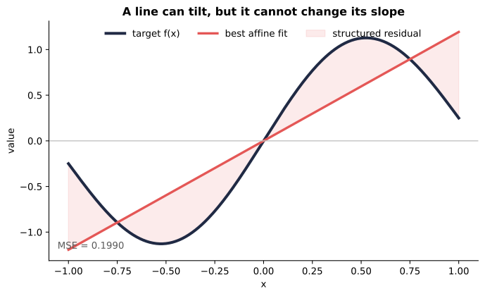
The fit in Figure 1 is already the least-squares solution for the displayed 241 training points. Its mean squared error is approximately \(0.1990\). Continuing to optimize the same two-parameter model cannot create the missing bends. The residual has structure because the model class is inadequate for this pattern.

This is a representation failure: no parameter choice within the affine family can express the required shape. An optimization failure is different. It occurs when a suitable parameter setting exists but the training procedure does not reach it—for example, because the learning rate is unstable or gradients become uninformative.

Important

An optimizer selects parameters within a model family. It does not enlarge that family. When every member of the family has constant slope, more optimization cannot produce changing slope.

The plotted error is a training residual. It tells us how the fitted line behaves on these displayed points; it is not validation evidence and does not establish how either model would generalize to new data. We will keep optimization and generalization as separate questions throughout the textbook.

We now need a component that can change slope. A neural network obtains that ability by placing nonlinear operations between affine transformations.

From an artificial neuron to nonlinear representation

Affine evidence followed by an activation

An artificial neuron receives \(d\) numerical inputs. It multiplies each input by a learned weight, adds the weighted contributions and a learned bias, and then applies an activation function:

\[ z =\mathbf w^\top\mathbf x+b =\sum_{j=1}^{d}w_jx_j+b, \qquad h=\phi(z). \]

The two named intermediate quantities have different roles:

• the preactivation \(z\) is an affine score;
• the activation \(h\) is the value passed to the next layer after applying \(\phi\).

Weights decide how strongly and in which direction each input contributes. The bias shifts the score before the activation is applied. The activation changes the form of the signal that later layers receive.

Common activations include sigmoid, hyperbolic tangent, and the rectified linear unit. We will use ReLU for the geometric examples:

\[ \operatorname{ReLU}(z)=\max(0,z) = \begin{cases} 0, & z\le0,\\ z, & z>0. \end{cases} \]

For one input, the neuron becomes

\[ h(x)=\operatorname{ReLU}(wx+b). \]

When \(w\ne0\), its affine score crosses zero at

\[ x_{\text{break}}=-\frac{b}{w}. \]

On one side of this breakpoint the neuron outputs zero. On the other side it outputs a line. The weight \(w\) controls the orientation and slope of the affine score, while \(b\) helps place the breakpoint.

Figure 2: A one-dimensional ReLU neuron first forms an affine preactivation, clips its negative side, and then contributes a scaled hinge to the output.

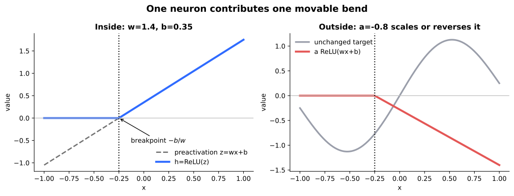
In Figure 2, the neuron does not reproduce the whole target. It supplies one simple geometric piece: a movable bend. A following layer can scale or reverse that piece with an output weight.

Why depth needs nonlinearity

Before combining several hinges, consider what happens if the activation is omitted. Let two successive layers be purely affine:

\[ \mathbf h=\mathbf W^{(1)}\mathbf x+\mathbf b^{(1)}, \qquad \mathbf y=\mathbf W^{(2)}\mathbf h+\mathbf b^{(2)}. \]

Substituting the first equation into the second gives

\[ \begin{aligned} \mathbf y &=\mathbf W^{(2)} \left(\mathbf W^{(1)}\mathbf x+\mathbf b^{(1)}\right) +\mathbf b^{(2)}\\ &=\left(\mathbf W^{(2)}\mathbf W^{(1)}\right)\mathbf x +\left(\mathbf W^{(2)}\mathbf b^{(1)}+\mathbf b^{(2)}\right). \end{aligned} \]

Define

\[ \widetilde{\mathbf W}=\mathbf W^{(2)}\mathbf W^{(1)}, \qquad \widetilde{\mathbf b} =\mathbf W^{(2)}\mathbf b^{(1)}+\mathbf b^{(2)}. \]

Then the entire two-layer calculation is simply

\[ \mathbf y=\widetilde{\mathbf W}\mathbf x+\widetilde{\mathbf b}. \]

Figure 3: Two affine layers collapse algebraically into one affine transformation with an equivalent weight matrix and bias vector.

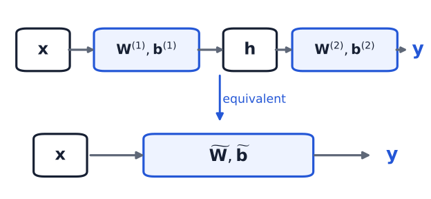
The same argument applies repeatedly: any finite composition of affine transformations is still affine. Extra parameter matrices may change how the same map is factorized, but they do not create a nonlinear input-output relationship. Nonlinear activations prevent the collapse shown in Figure 3.

Several hinges form a richer function

Let a hidden layer contain \(H\) ReLU neurons that receive the same scalar input. A linear output layer combines their activations:

\[ h_j(x)=\operatorname{ReLU}(w_jx+b_j), \qquad \hat f(x)=b_2+\sum_{j=1}^{H}a_jh_j(x). \]

Each pair \((w_j,b_j)\) positions and orients a hinge. Each output weight \(a_j\) scales or reverses that hinge’s contribution. The final bias \(b_2\) moves the complete sum vertically.

Figure 4: Four ReLU hinge contributions and an output bias combine into a continuous piecewise-linear approximation of the smooth target.

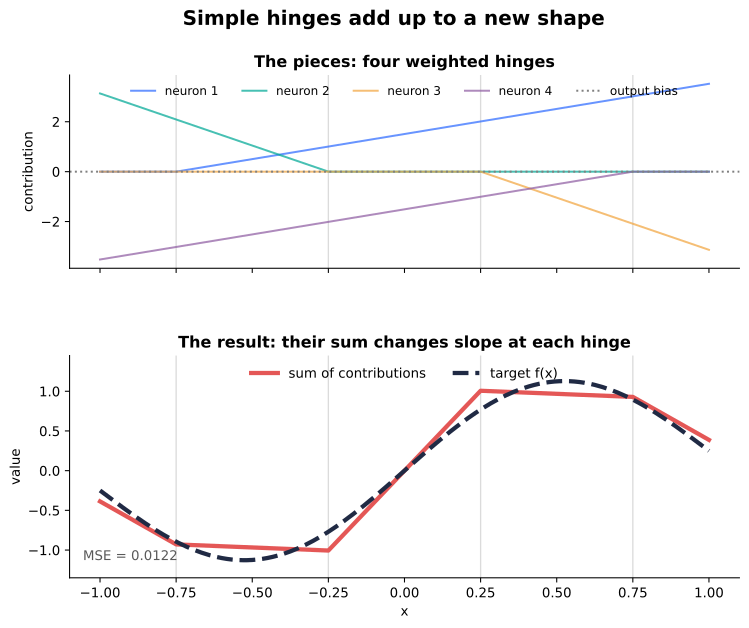
Between neighboring breakpoints, the active set of neurons does not change. Every active contribution is affine on that interval, so their sum is also affine there. At a breakpoint, one neuron’s state changes and the total slope may change. The result in Figure 4 is therefore continuous and piecewise linear.

This explanation is deliberately more modest than a universal-approximation theorem. The figure reveals the mechanism needed here: several simple nonlinear components create a family of functions that a single affine model cannot represent.

Important

PyTorch’s nn.Linear computes the affine part \(\mathbf W\mathbf x+\mathbf b\). Despite its name, the inclusion of a bias makes this an affine map in mathematical terminology. ReLU or another activation is a separate operation.

The next step is to collect parallel neurons into vectors and make their dimensions explicit.

Layers, tensor shapes, and forward propagation

From one neuron to a layer

Suppose layer \(\ell\) has width \(d_\ell\) and receives a vector with \(d_{\ell-1}\) components. Each output neuron has its own row of weights and its own bias. For one sample, define

\[ \mathbf h^{(0)}=\mathbf x, \]

and for each subsequent layer,

\[ \mathbf z^{(\ell)} =\mathbf W^{(\ell)}\mathbf h^{(\ell-1)} +\mathbf b^{(\ell)}, \qquad \mathbf h^{(\ell)} =\phi_\ell\!\left(\mathbf z^{(\ell)}\right). \]

The activation is applied elementwise unless stated otherwise. The shapes are

\[ \mathbf h^{(\ell-1)}\in\mathbb R^{d_{\ell-1}}, \qquad \mathbf W^{(\ell)}\in \mathbb R^{d_\ell\times d_{\ell-1}}, \]

\[ \mathbf b^{(\ell)},\mathbf z^{(\ell)},\mathbf h^{(\ell)} \in\mathbb R^{d_\ell}. \]

Row \(j\) of \(\mathbf W^{(\ell)}\) contains the weights of output neuron \(j\). Multiplying that row by \(\mathbf h^{(\ell-1)}\) produces the neuron’s weighted sum. Collecting all rows evaluates every neuron in the layer in one matrix operation.

One sample and a row-major batch

The preceding equations use column vectors because they make the calculation for one sample easy to read. PyTorch normally stores a batch of \(B\) samples in the rows of a matrix:

\[ \mathbf H^{(\ell-1)} \in\mathbb R^{B\times d_{\ell-1}}. \]

PyTorch still stores the weight matrix as

\[ \mathbf W^{(\ell)} \in\mathbb R^{d_\ell\times d_{\ell-1}}, \]

so the batch equation uses its transpose:

\[ \mathbf Z^{(\ell)} =\mathbf H^{(\ell-1)}\mathbf W^{(\ell)\top} +\mathbf b^{(\ell)} \in\mathbb R^{B\times d_\ell}. \]

The multiplication has the shape

\[ (B\times d_{\ell-1}) (d_{\ell-1}\times d_\ell) =B\times d_\ell. \]

The bias has shape \((d_\ell,)\). It is reused for every sample row: PyTorch broadcasts it as though the same bias vector had been added to all \(B\) rows. No separate bias parameter is learned for each sample.

Figure 5: For a batch-first linear layer, a batch-by-input-width matrix multiplies the transpose of the stored output-by-input weight matrix; one output-width bias broadcasts across the rows.

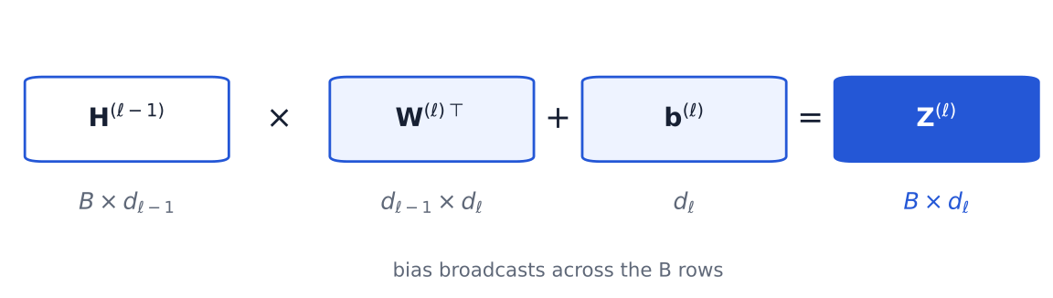
Figure 5 is not merely bookkeeping. A mismatched shape often reveals a mistaken interpretation of which axis represents samples, input features, or output neurons.

Worked example: a complete \(2\to3\to1\) forward pass

Take one input with two features:

\[ \mathbf x= \begin{bmatrix} 2\\-1 \end{bmatrix}. \]

The first layer has three ReLU neurons:

\[ \mathbf W^{(1)}= \begin{bmatrix} 0.5&1\\ -1&0.5\\ 1&1 \end{bmatrix}, \qquad \mathbf b^{(1)}= \begin{bmatrix} 0.5\\0\\-0.5 \end{bmatrix}. \]

The three preactivations are

\[ \begin{aligned} \mathbf z^{(1)} &=\mathbf W^{(1)}\mathbf x+\mathbf b^{(1)}\\ &= \begin{bmatrix} 0.5(2)+1(-1)+0.5\\ -1(2)+0.5(-1)+0\\ 1(2)+1(-1)-0.5 \end{bmatrix}\\ &= \begin{bmatrix} 0.5\\-2.5\\0.5 \end{bmatrix}. \end{aligned} \]

Applying ReLU elementwise gives

\[ \mathbf h^{(1)} =\operatorname{ReLU}(\mathbf z^{(1)}) = \begin{bmatrix} 0.5\\0\\0.5 \end{bmatrix}. \]

The second layer is an affine output layer; equivalently, its activation is the identity:

\[ \mathbf W^{(2)}= \begin{bmatrix} 2&-1&1 \end{bmatrix}, \qquad b^{(2)}=-0.5. \]

Therefore

\[ \begin{aligned} \hat y &=\mathbf W^{(2)}\mathbf h^{(1)}+b^{(2)}\\ &=2(0.5)-1(0)+1(0.5)-0.5\\ &=1. \end{aligned} \]

Figure 6: The checked two-to-three-to-one network carries the input values through three hidden preactivations, ReLU activations, and a final affine output to produce one.

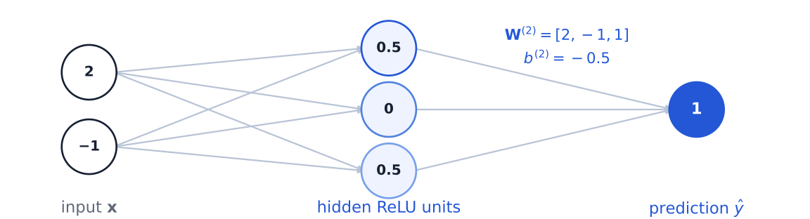
The calculation in Figure 6 is forward propagation: evaluate each operation in dependency order, using the parameters as they currently are. No learning occurs during this pass.

Reading nn.Linear as mathematics

For a batch X with shape (B, 2), PyTorch’s nn.Linear(2, 3) stores weight with shape (3, 2) and bias with shape (3,). Its output has shape (B, 3) (PyTorch contributors, n.d.-d). The following self-contained shape check uses \(B=4\); the same algebra holds for any batch size:

import torch
from torch import nn

B = 4
X = torch.zeros(B, 2)
layer = nn.Linear(in_features=2, out_features=3)

Z = layer(X)
Z_explicit = X @ layer.weight.T + layer.bias

torch.testing.assert_close(Z, Z_explicit)
assert Z.shape == (X.shape[0], 3)

The transpose is required because samples occupy rows of X while output units occupy rows of layer.weight. The bias broadcasts over the batch dimension. The layer does not apply ReLU:

H = torch.relu(layer(X))

These two lines represent two distinct mathematical operations. Keeping them distinct becomes essential when we later ask which intermediate values must be remembered and how sensitivities move backward through the same sequence.

Forward propagation has now given us a precise answer to the first question of neural-network training: what prediction does this parameterized composition produce for these inputs?

From network outputs to a learning objective

The output layer has a job-specific meaning

Forward propagation ends with numbers, but their meaning is not determined by the network architecture alone. The task determines how the final layer is interpreted and how its output is compared with the target. Three common cases provide the operational pattern we need.

Task	Final-layer output	Interpretation and typical loss
Regression	One or more unconstrained values	Predictions in the target’s units; mean squared error is appropriate when squared error matches the modeling objective.
Binary classification	One unconstrained logit \(z_i\)	Probability \(q_i=\sigma(z_i)\); binary cross-entropy computed directly from logits is the numerically stable interface.
Multiclass classification	\(K\) unconstrained logits \(z_{i1},\ldots,z_{iK}\)	Softmax probabilities over mutually exclusive classes; cross-entropy uses the observed class.

For regression, an identity output activation leaves the prediction unconstrained. The loss need not always be squared error—absolute error and task-specific losses are possible—but the output must have the meaning and shape expected by the chosen loss.

For binary classification, the single logit is not itself a probability. Applying the sigmoid gives a number between zero and one. In PyTorch, binary_cross_entropy_with_logits or nn.BCEWithLogitsLoss accepts the raw logit and combines the sigmoid and binary cross-entropy calculation. This avoids forming probabilities in a less stable sequence of separate operations (PyTorch contributors, n.d.-b).

For multiclass classification, one example \(i\) receives \(K\) logits. Write the logit for class \(k\) as \(z_{ik}\). Softmax turns the vector of logits into probabilities:

\[ q_{ik} = \frac{\exp z_{ik}} {\sum_j \exp z_{ij}}. \]

The probabilities are positive and sum to one. They preserve the ordering of the logits: the largest logit corresponds to the largest probability.

Figure 7: Softmax exponentiates a vector of class logits and normalizes the resulting positive values into probabilities that sum to one.

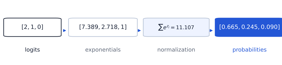
Figure 7 separates two objects that are easy to conflate: the network emits logits, while Softmax normalizes them into probabilities. The target is not an input to Softmax; it enters afterward, when the loss identifies which class probability was observed.

Softmax depends on relative rather than absolute logit levels. Adding the same constant \(r\) to every logit leaves every probability unchanged:

\[ \frac{\exp(z_{ik}+r)}{\sum_j\exp(z_{ij}+r)} = \frac{\exp(r)\exp(z_{ik})} {\exp(r)\sum_j\exp(z_{ij})} =q_{ik}. \]

Stable implementations use this identity to subtract a convenient constant, commonly the largest logit, before exponentiating. The identity also explains why an argmax decision does not require Softmax:

\[ \operatorname*{arg\,max}_k z_{ik} = \operatorname*{arg\,max}_k q_{ik}. \]

Softmax probabilities matter when we need a probabilistic output or a probability-based loss. Whether those probabilities are calibrated is a separate empirical question. They do not change which class has the largest score.

Cross-entropy and the target convention

Let \(c_i\) be the observed class index for example \(i\), and let \(y_{ik}\) be the corresponding one-hot entry: \(y_{ik}=1\) for the observed class and \(0\) otherwise. The per-example multiclass cross-entropy can be written in two equivalent ways:

\[ \ell_i = -\log q_{i,c_i} = -\sum_k y_{ik}\log q_{ik}. \]

The first form selects the observed class by its integer index. The second uses a one-hot vector to perform the same selection. These are two representations of the same target, not two different observed classes.

For the checked logits

\[ [2,1,0], \]

Softmax gives

\[ [2,1,0] \longmapsto [0.665241,\;0.244728,\;0.090031]. \]

Suppose the observed category is the second class when classes are named from one. Its probability is \(0.244728\), so

\[ \ell=-\log(0.244728)\approx1.407606. \]

Important

“Second class” is pedagogical one-based naming. PyTorch class indices are zero-based, so the integer target for that class is 1, not 2. Its one-hot representation is \([0,1,0]\). Thus all three statements below refer to exactly the same category:

• human-facing name: class 2;
• PyTorch class-index target: 1;
• one-hot target: \([0,1,0]\).

For a batch of \(B\) examples and \(K\) classes, the usual PyTorch interface is

import torch.nn.functional as F

# logits: (B, K)
# targets: (B,) of dtype torch.long
loss = F.cross_entropy(logits, targets)

F.cross_entropy receives logits, not probabilities produced by a preceding Softmax. With class-index targets, it combines log-softmax and negative log-likelihood in a numerically stable calculation. For the unweighted batch here, with no ignored targets, its default reduction is the mean over the batch; other reductions can be requested explicitly. The official documentation specifies the accepted input and target shapes and the more general weighted reduction behavior (PyTorch contributors, n.d.-c).

This compact treatment tells us how to construct a scalar objective without repeating the full categorical-likelihood, maximum-likelihood, entropy, and KL-divergence development that belongs in the Week 07 chapter. We now have the question that drives backpropagation: once the scalar loss is known, how does every connected parameter receive its own sensitivity?

Backpropagation begins with a scalar computation graph

One calculation, exposed node by node

A formula such as \(L(f_\theta(x),y)\) hides the intermediate values through which the loss depends on a parameter. A computation graph exposes those dependencies. Consider the canonical scalar network

\[ z=wx+b, \qquad h=\operatorname{ReLU}(z), \qquad \hat y=ah+c, \qquad L=\frac12(\hat y-y)^2. \]

Use the checked values

\[ x=3,\quad y=2,\quad w=2,\quad b=-1,\quad a=0.4,\quad c=-1. \]

The forward pass evaluates each node only after its inputs are known: \(z=5\), \(h=5\), \(\hat y=1\), and \(L=0.5\).

Figure 8: The scalar network’s forward computation evaluates an affine hidden score, ReLU activation, affine prediction, and squared-error loss in dependency order.

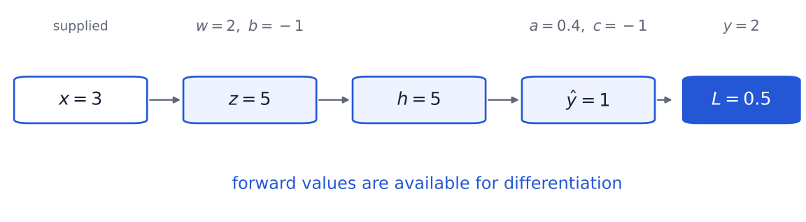
Figure 8 is the same model as the four equations, but it records which value each later operation needs. Backpropagation traverses these dependencies in reverse.

Local derivatives and incoming sensitivities

A gradient is a local sensitivity. For example, \(\partial L/\partial w\) describes the first-order change in the current loss caused by a small change in the current value of \(w\), with the other inputs held fixed. It is not itself a parameter update.

Start at the scalar loss with the seed

\[ \frac{\partial L}{\partial L}=1. \]

Each node receives an incoming sensitivity from operations closer to the loss, multiplies by its own local derivative, and passes the result to its inputs. The single cumulative ledger below records every supplied or computed forward value together with the complete reverse pass. The target \(y\) is included for completeness, although it is observed rather than optimized.

Node	Forward value	Incoming sensitivity	Local derivative	Resulting sensitivity
\(L\)	\(0.5\)	—	\(\partial L/\partial L=1\)	loss seed \(1\)
\(\hat y\)	\(1\)	\(1\)	\(\partial L/\partial\hat y=\hat y-y=-1\)	\(\partial L/\partial\hat y=-1\)
\(y\)	\(2\) (target)	\(1\)	\(\partial L/\partial y=y-\hat y=1\)	\(\partial L/\partial y=1\)
\(a\)	\(0.4\)	\(\partial L/\partial\hat y=-1\)	\(\partial\hat y/\partial a=h=5\)	\(\partial L/\partial a=-5\)
\(c\)	\(-1\)	\(\partial L/\partial\hat y=-1\)	\(\partial\hat y/\partial c=1\)	\(\partial L/\partial c=-1\)
\(h\)	\(5\)	\(\partial L/\partial\hat y=-1\)	\(\partial\hat y/\partial h=a=0.4\)	\(\partial L/\partial h=-0.4\)
\(z\)	\(5\)	\(\partial L/\partial h=-0.4\)	\(\partial h/\partial z=1\) because \(z>0\)	\(\partial L/\partial z=-0.4\)
\(w\)	\(2\)	\(\partial L/\partial z=-0.4\)	\(\partial z/\partial w=x=3\)	\(\partial L/\partial w=-1.2\)
\(b\)	\(-1\)	\(\partial L/\partial z=-0.4\)	\(\partial z/\partial b=1\)	\(\partial L/\partial b=-0.4\)
\(x\)	\(3\)	\(\partial L/\partial z=-0.4\)	\(\partial z/\partial x=w=2\)	\(\partial L/\partial x=-0.8\)

Figure 9: The complete reverse pass annotates every edge of the scalar computation graph with its local derivative and every node with the resulting loss sensitivity.

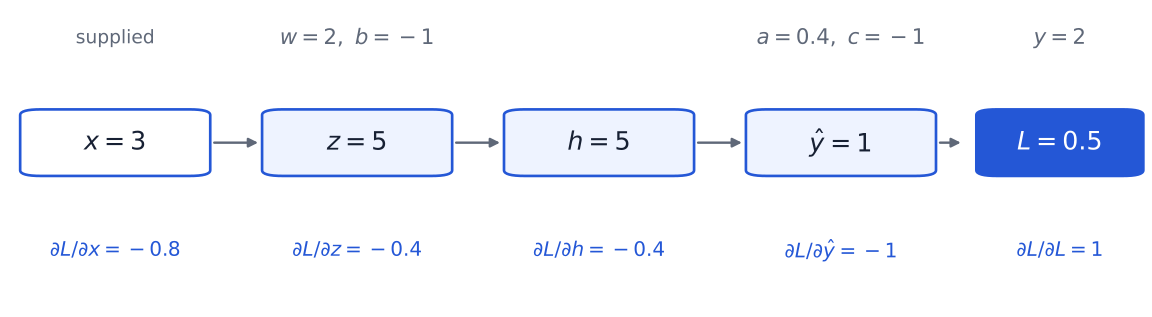
The two highlighted endpoint results in Figure 9 are

\[ \frac{\partial L}{\partial w}=-1.2, \qquad \frac{\partial L}{\partial x}=-0.8. \]

The derivative with respect to \(x\) matters even though \(x\) is not a trainable parameter in this example: an earlier layer would treat this value as its incoming sensitivity. Reverse propagation therefore uses the same rule for trainable parameters and intermediate activations; the optimizer later decides which trainable leaves to update.

Why paths multiply and branches add

Along a single path, the chain rule multiplies local rates of change. For \(w\), the only path to the loss is

\[ w\longrightarrow z\longrightarrow h\longrightarrow\hat y\longrightarrow L, \]

so

\[ \frac{\partial L}{\partial w} = \frac{\partial L}{\partial\hat y} \frac{\partial\hat y}{\partial h} \frac{\partial h}{\partial z} \frac{\partial z}{\partial w} =(-1)(0.4)(1)(3)=-1.2. \]

Each factor answers what a small change does at one edge. Their product answers what a small change in \(w\) does after passing through the complete dependency chain.

When one value affects the loss along several outgoing paths, the total first-order effect is the sum of the path contributions. In the smallest useful branch example, suppose \(u_1=rh\), \(u_2=sh\), and \(L=L_1(u_1)+L_2(u_2)\). Then

\[ \frac{\partial L}{\partial h} = \frac{\partial L_1}{\partial u_1}r + \frac{\partial L_2}{\partial u_2}s. \]

This addition is not an extra backpropagation convention. It is the multivariable chain rule accounting for every route by which \(h\) influences \(L\). The bias-gradient sum across a batch in the next section is the same branching principle.

ReLU controls whether an upstream path is active:

\[ \frac{d}{dz}\operatorname{ReLU}(z) = \begin{cases} 0,&z<0,\\ 1,&z>0. \end{cases} \]

Here \(z=5\), so the sensitivity passes through unchanged. If \(z<0\), the local derivative is zero and every gradient farther upstream on that path becomes zero. Such a zero gradient can mean that this particular ReLU path is inactive for this input; it does not by itself show that the model has converged. ReLU is nondifferentiable at exactly zero. PyTorch’s documented minimum-norm subgradient rule selects zero at that point (PyTorch contributors, n.d.-a).

An independent numerical check

A central finite difference estimates the derivative without using the backward ledger. Holding every other value fixed and choosing \(\varepsilon=10^{-5}\),

\[ \frac{L(w+\varepsilon)-L(w-\varepsilon)}{2\varepsilon} = \frac{0.499988000072-0.500012000072}{2\times10^{-5}} =-1.200000000021. \]

This agrees with \(\partial L/\partial w=-1.2\) to numerical precision. A finite difference is useful as a check, but it requires new forward evaluations for each perturbed parameter. Backpropagation obtains all connected sensitivities in one reverse traversal.

The step size balances two errors. If \(\varepsilon\) is too large, the finite interval is a poor approximation to the local derivative; if it is too small, subtracting nearly equal floating-point losses magnifies roundoff. A check should therefore use a stated absolute or relative tolerance rather than demand bitwise equality. At a smooth point in a short float64 calculation, tolerances around \(10^{-5}\) are often a reasonable starting check, but the appropriate value depends on scale and numerical depth. A perturbation that crosses a ReLU breakpoint compares different linear regions, so disagreement there need not indicate an incorrect backward rule.

Backpropagation stops after computing these gradients. A rule such as \(w\leftarrow w-\eta\,\partial L/\partial w\) is a separate optimization step. The Ode to Autograd tutorial provides an independent scalar practice graph with different numerical values; those values should not be mixed with this canonical calculation.

From scalar derivatives to matrix backpropagation

A batched affine-plus-activation layer

The scalar graph scales to a layer by applying the same local chain-rule logic to arrays. Use the established batch-row convention for a layer with batch size \(B\), input width \(d_{\mathrm{in}}\), and output width \(d_{\mathrm{out}}\):

\[ \mathbf Z = \mathbf H_{\mathrm{in}}\mathbf W^\top+\mathbf b, \qquad \mathbf H=\phi(\mathbf Z). \]

The shapes are

\[ \mathbf H_{\mathrm{in}}\in\mathbb R^{B\times d_{\mathrm{in}}}, \quad \mathbf W\in\mathbb R^{d_{\mathrm{out}}\times d_{\mathrm{in}}}, \quad \mathbf b\in\mathbb R^{d_{\mathrm{out}}}, \]

\[ \mathbf Z,\mathbf H\in\mathbb R^{B\times d_{\mathrm{out}}}. \]

Assume the rest of the network and the loss have already produced the incoming sensitivity

\[ \mathbf G_H = \frac{\partial L}{\partial\mathbf H} \in\mathbb R^{B\times d_{\mathrm{out}}}. \]

For an elementwise activation, the first backward operation is also elementwise:

\[ \mathbf G_Z = \mathbf G_H\odot\phi'(\mathbf Z) \in\mathbb R^{B\times d_{\mathrm{out}}}. \]

For ReLU, \(\phi'(\mathbf Z)\) is a pass/block mask. An entry with positive preactivation passes its incoming sensitivity; an entry with negative preactivation blocks it.

Figure 10: Three examples produce different positive and negative preactivations in the same ReLU layer, so each row has its own pass/block mask.

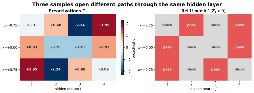
Figure 10 makes one important point visible: a shared layer can expose different active paths for different sample rows. The derivative mask therefore has the same \(B\times d_{\mathrm{out}}\) shape as the preactivation and the incoming sensitivity.

Derive one weight entry before writing the matrix rule

The \((i,j)\) preactivation is

\[ Z_{ij} = \sum_{k=1}^{d_{\mathrm{in}}} H_{\mathrm{in},ik}W_{jk}+b_j. \]

The parameter \(W_{jk}\) is shared across all \(B\) sample rows. For a particular row \(i\),

\[ \frac{\partial Z_{ij}}{\partial W_{jk}} =H_{\mathrm{in},ik}. \]

Its total influence on the scalar loss adds the contributions from every row:

\[ \frac{\partial L}{\partial W_{jk}} = \sum_{i=1}^{B} \frac{\partial L}{\partial Z_{ij}} \frac{\partial Z_{ij}}{\partial W_{jk}} = \sum_{i=1}^{B} G_{Z,ij}H_{\mathrm{in},ik}. \]

This is the \((j,k)\) entry of a matrix product: row \(j\) of \(\mathbf G_Z^\top\) contains \(G_{Z,1j},\ldots,G_{Z,Bj}\), while column \(k\) of \(\mathbf H_{\mathrm{in}}\) contains \(H_{\mathrm{in},1k},\ldots,H_{\mathrm{in},Bk}\). Collecting every \((j,k)\) entry gives

\[ \frac{\partial L}{\partial\mathbf W} = \mathbf G_Z^\top\mathbf H_{\mathrm{in}} \in\mathbb R^{d_{\mathrm{out}}\times d_{\mathrm{in}}}. \]

The transpose is required by both meaning and shape:

\[ (d_{\mathrm{out}}\times B) (B\times d_{\mathrm{in}}) =d_{\mathrm{out}}\times d_{\mathrm{in}}, \]

which matches the stored weight matrix.

Each bias \(b_j\) also affects output \(j\) in every sample row, with local derivative one. Its gradient therefore sums across the batch axis:

\[ \frac{\partial L}{\partial\mathbf b} = \sum_{i=1}^{B}\mathbf G_{Z,i} \in\mathbb R^{d_{\mathrm{out}}}. \]

Finally, the sensitivity passed to the preceding layer is

\[ \frac{\partial L}{\partial\mathbf H_{\mathrm{in}}} = \mathbf G_Z\mathbf W \in\mathbb R^{B\times d_{\mathrm{in}}}, \]

because

\[ (B\times d_{\mathrm{out}}) (d_{\mathrm{out}}\times d_{\mathrm{in}}) =B\times d_{\mathrm{in}}. \]

Figure 11: Backward propagation through one batched affine-plus-activation layer first applies the activation derivative, then forms parameter gradients and the sensitivity for the preceding layer.

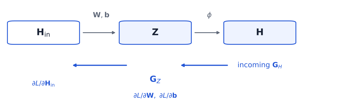
The three routes in Figure 11 are the array versions of the scalar graph. Multiplication follows each dependency path; shared parameters collect contributions from all paths that meet them.

A small batch with different active paths

Take \(B=3\), \(d_{\mathrm{in}}=2\), and \(d_{\mathrm{out}}=2\):

\[ \mathbf H_{\mathrm{in}}= \begin{bmatrix} 1&0\\ 0&1\\ 1&1 \end{bmatrix}. \]

\[ \mathbf W= \begin{bmatrix} 1&-1\\ -1&2 \end{bmatrix}, \qquad \mathbf b= \begin{bmatrix} 0.2&0.5 \end{bmatrix}. \]

The forward preactivations and ReLU mask are

\[ \mathbf Z= \begin{bmatrix} 1.2&-0.5\\ -0.8&2.5\\ 0.2&1.5 \end{bmatrix}, \qquad \phi'(\mathbf Z)= \begin{bmatrix} 1&0\\ 0&1\\ 1&1 \end{bmatrix}. \]

The first example activates only output path 1, the second activates only path 2, and the third activates both. Suppose the incoming sensitivity is

\[ \mathbf G_H= \begin{bmatrix} 1&2\\ -1&1\\ 0.5&-2 \end{bmatrix}. \]

Applying the mask gives

\[ \mathbf G_Z = \begin{bmatrix} 1&0\\ 0&1\\ 0.5&-2 \end{bmatrix}. \]

The layer gradients are then

\[ \frac{\partial L}{\partial\mathbf W} = \begin{bmatrix} 1.5&0.5\\ -2&-1 \end{bmatrix}. \]

\[ \frac{\partial L}{\partial\mathbf b} = \begin{bmatrix} 1.5&-1 \end{bmatrix}, \]

\[ \frac{\partial L}{\partial\mathbf H_{\mathrm{in}}} = \begin{bmatrix} 1&-1\\ -1&2\\ 2.5&-4.5 \end{bmatrix}. \]

The bias result makes the reduction visible. Its first entry is \(1+0+0.5=1.5\), and its second is \(0+1-2=-1\). A bias is reused in each row during the forward pass, so its backward contributions must be added across those rows.

Sum, mean, and repeated local rules

The formulas above do not silently choose a loss reduction. They assume that \(\mathbf G_H\) is the derivative of the actual scalar loss \(L\) supplied to the layer. If

\[ L_{\mathrm{sum}}=\sum_{i=1}^{B}\ell_i, \]

then the incoming sensitivity contains derivatives of that sum. If instead

\[ L_{\mathrm{mean}}=\frac1B\sum_{i=1}^{B}\ell_i, \]

then every per-example contribution in the incoming sensitivity already contains the factor \(1/B\). The layer formulas remain unchanged; for the same batch, gradients of the mean are \(1/B\) times the corresponding gradients of the sum.

For a multilayer perceptron, these local rules simply repeat in reverse layer order. At layer \(\ell\), compute

\[ \mathbf G_Z^{(\ell)} = \mathbf G_H^{(\ell)}\odot \phi_\ell'(\mathbf Z^{(\ell)}), \]

use it to obtain the gradients of \(\mathbf W^{(\ell)}\) and \(\mathbf b^{(\ell)}\), and pass

\[ \mathbf G_H^{(\ell-1)} = \mathbf G_Z^{(\ell)}\mathbf W^{(\ell)} \]

to the preceding layer. For an affine output layer with the identity activation, the activation derivative is one, so \(\mathbf G_Z=\mathbf G_H\) there.

Figure 12: An MLP backward pass applies the same activation, parameter-gradient, and input-sensitivity rules repeatedly from the scalar loss toward earlier layers.

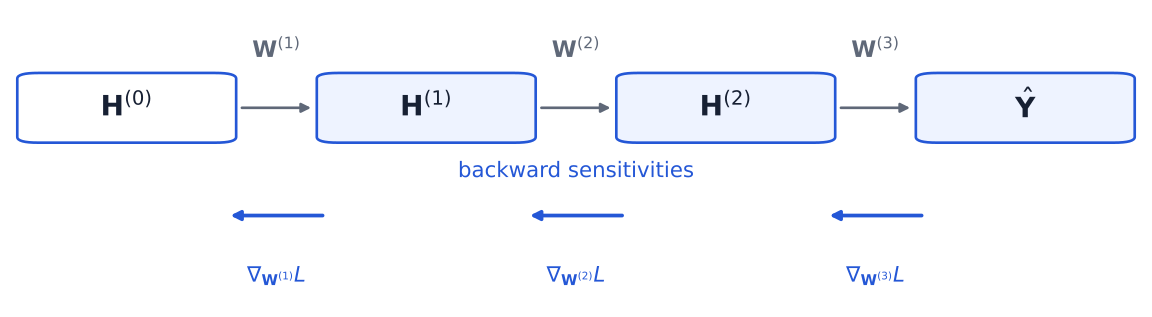
Each multiplication by a local derivative is a vector–Jacobian product: it combines the sensitivity arriving from later computations with the local derivative of the current operation. Backpropagation evaluates these products directly. It does not need to construct and store a full Jacobian matrix for every layer. Figure 12 therefore represents one repeated principle, not a separate formula for every possible architecture.

The scalar ledger and the matrix identities now describe what reverse-mode differentiation must compute. The companion tutorial checks the same local rules against PyTorch autograd. Together they provide a testable mathematical specification for an automatic implementation.

Autograd as an implementation of the mathematics

The same reverse pass, recorded automatically

PyTorch autograd implements the reverse-mode differentiation developed in the previous two sections. When gradient recording is enabled, the forward pass does two jobs: it computes tensor values and records the operations and dependencies needed for a later reverse pass. Calling backward() on a scalar loss then supplies the familiar seed

\[ \frac{\partial L}{\partial L}=1 \]

and traverses the recorded graph in reverse. At each operation, autograd applies the operation’s local vector–Jacobian product. Connected leaf tensors that require gradients receive the accumulated sensitivities in their .grad attributes (PyTorch contributors, n.d.-a).

Nothing about this changes the mathematics. Autograd automates the bookkeeping that would otherwise fill the scalar ledger or repeat the layer rules. It does not decide which model represents the task, which loss expresses the objective, which optimizer should use the gradients, or what scientific conclusion the resulting experiment supports.

The canonical scalar example can be written almost line for line in PyTorch:

import torch

x = torch.tensor(3.0, requires_grad=True)
w = torch.tensor(2.0, requires_grad=True)
b = torch.tensor(-1.0, requires_grad=True)
a = torch.tensor(0.4, requires_grad=True)
c = torch.tensor(-1.0, requires_grad=True)
y = torch.tensor(2.0)

z = w * x + b
h = torch.relu(z)
y_hat = a * h + c
loss = 0.5 * (y_hat - y) ** 2
loss.backward()

actual = torch.stack([a.grad, c.grad, w.grad, b.grad, x.grad])
expected = torch.tensor([-5.0, -1.0, -1.2, -0.4, -0.8])
torch.testing.assert_close(actual, expected)

The last assertion checks all five manual results. In particular, w.grad is \(-1.2\) and x.grad is \(-0.8\). The call to loss.backward() has populated gradients; it has not changed any of the values \(w,b,a,c\).

Leaves, intermediates, and stored gradients

Setting requires_grad=True tells autograd that operations involving a tensor may need to participate in reverse-mode differentiation. In the example, \(x,w,b,a,c\) are leaf tensors: they were created directly rather than produced by a recorded operation. The tensors z, h, y_hat, and loss are non-leaf tensors produced inside the graph.

Trainable nn.Parameter objects are normally leaves for the same practical reason. The optimizer needs a stable set of tensors whose .grad fields it can inspect. Non-leaf gradients are still calculated as sensitivities pass through the graph, but PyTorch does not retain them in .grad by default. Thus after the preceding example:

assert w.is_leaf and w.grad is not None
assert not z.is_leaf
z.grad  # None by default; PyTorch may also emit a reminder warning

This does not mean the gradient through z was skipped: the nonzero values in w.grad, b.grad, and x.grad could not have been produced without it. If an intermediate gradient is needed for diagnosis, call retain_grad() on that non-leaf tensor before the reverse pass (PyTorch contributors, n.d.-g):

for tensor in (x, w, b, a, c):
    tensor.grad = None

z_check = w * x + b
z_check.retain_grad()
h_check = torch.relu(z_check)
loss_check = 0.5 * (a * h_check + c - y) ** 2
loss_check.backward()

torch.testing.assert_close(z_check.grad, torch.tensor(-0.4))

Retaining every intermediate gradient would consume memory without helping a routine training update, so it is best treated as a targeted inspection tool.

Accumulation is deliberate

Within one backward pass, autograd sums contributions from all graph paths according to the chain rule. Across separate backward calls, PyTorch adds the newly computed leaf gradient to any value already stored in .grad. The first behavior is required by the computation graph; the second enables deliberate accumulation across mini-batches and is why gradients normally must be cleared before a new update.

The following example isolates the second behavior. w.grad already contains the gradient from loss_check.backward(). A new forward pass builds a new graph for the same calculation, and a separate backward call adds its newly computed gradient to the stored value:

first_w_grad = w.grad.clone()

# Recompute the forward pass because the first graph was released.
loss_again = 0.5 * (a * torch.relu(w * x + b) + c - y) ** 2
loss_again.backward()

torch.testing.assert_close(w.grad, 2 * first_w_grad)

for tensor in (x, w, b, a, c):
    tensor.grad = None
assert all(tensor.grad is None for tensor in (x, w, b, a, c))

The forward pass is recomputed because a normal backward call releases graph information after using it. The second call therefore contributes another \(-1.2\) to w.grad, making the stored value \(-2.4\). Clearing gradients restores the intended starting condition for a new training update. Model training usually delegates that clearing to optimizer.zero_grad() (PyTorch contributors, n.d.-e).

Cutting a dependency with detach()

Sometimes a value should be reused numerically without allowing a later loss to send sensitivity through its earlier history. Calling detach() returns a tensor disconnected from the graph that produced it. It is not merely a data copy: the returned tensor shares storage with its source, so in-place changes can be visible on both. Nor does detaching one tensor put a model into evaluation mode (PyTorch contributors, n.d.-f).

In the scalar network, detaching \(h\) blocks the route to \(z,w,b,x\), while the later leaves \(a\) and \(c\) remain connected:

for tensor in (x, w, b, a, c):
    tensor.grad = None

z_cut = w * x + b
h_cut = torch.relu(z_cut).detach()
loss_cut = 0.5 * (a * h_cut + c - y) ** 2
loss_cut.backward()

assert w.grad is None and b.grad is None and x.grad is None
torch.testing.assert_close(a.grad, torch.tensor(-5.0))
torch.testing.assert_close(c.grad, torch.tensor(-1.0))

The result is a graph statement, not a claim that the upstream numerical calculation disappeared: h_cut still equals \(5\).

Three commonly confused controls act at different levels:

Control	What it changes	What it does not do
tensor.detach()	Returns a tensor that shares storage with its source but is cut from the source’s previous autograd history.	Does not change a model’s training or evaluation behavior.
with torch.no_grad():	Prevents ordinary operations in the context from being recorded for reverse-mode differentiation.	Does not switch the model from training behavior to evaluation behavior.
model.eval()	Switches modules that define distinct evaluation behavior.	Does not globally disable gradient recording.

For validation, the usual combination is therefore model.eval() and a no-grad context. The first selects appropriate module behavior; the second avoids constructing an unnecessary backward graph. Returning to training requires model.train(). These controls are orthogonal in PyTorch’s documented semantics (PyTorch contributors, n.d.-a).

Figure 13: For a checked layer, manual matrix backpropagation and PyTorch autograd place markers at exactly the same parameter-gradient values.

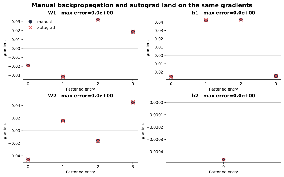
Figure 13 verifies the same principle at layer scale: autograd’s answers agree with the explicit matrix rules, entry by entry. The Ode to Autograd tutorial develops the full executable sequence, including inactive ReLU paths and additional checks. The chapter’s purpose is the contract behind that code: backward() computes and accumulates sensitivities, while a separate optimizer may later use them.

From gradients to a training process

One update in seven steps

A correct gradient describes local loss sensitivity at the current parameters. Learning requires using such gradients repeatedly. One training update has the following conceptual order:

1. select a mini-batch of inputs and targets;
2. clear parameter gradients left by earlier updates;
3. run forward propagation;
4. reduce the example losses to one scalar loss;
5. run backpropagation;
6. update the parameters;
7. record training diagnostics and, according to a chosen schedule, evaluate on validation data.

The computational core is compact:

optimizer.zero_grad()
prediction = model(X)
loss = criterion(prediction, y)
loss.backward()
optimizer.step()

Each line has a distinct role. zero_grad() clears accumulated parameter sensitivities. model(X) evaluates the current parameterized function. criterion(...) turns its predictions and targets into the scalar objective for this batch. backward() computes and stores parameter gradients. Only step() changes the parameters, following the optimizer’s update rule and current state.

Writing optimizer.zero_grad(set_to_none=True) explicitly is a common form. It leaves absent gradients as None until the next backward pass rather than filling existing buffers with zeros; this can reduce memory operations, and optimizers may distinguish a missing gradient from a zero-valued one. The central requirement is unchanged: old contributions must not silently enter a new update unless accumulation is intentional.

Training diagnostics belong after the quantities they report exist. Batch loss can be recorded after the forward pass; gradient diagnostics require the backward pass; parameter diagnostics may be recorded before or after step() as long as that choice is named. Validation normally occurs at a less frequent schedule than every update and must not update the parameters.

Mini-batches estimate a full-data direction

Let \(\mathcal B_t\) be the set of example indices selected at update step \(t\). With a mean reduction, its scalar loss is

\[ L_{\mathcal B_t} = \frac{1}{|\mathcal B_t|} \sum_{i\in\mathcal B_t}\ell_i. \]

The update can be summarized as

\[ \theta_{t+1} = \theta_t - \eta\, \widehat{\nabla_\theta L}_{\mathcal B_t}. \]

The hat emphasizes that the mini-batch gradient estimates the full-dataset gradient. It is not an incorrect gradient: it is exactly the gradient of the selected mini-batch objective, used as a computationally affordable, stochastic direction for the larger training objective.

Figure 14: At the same parameter value, gradients from different mini-batches vary around the direction obtained from all training examples.

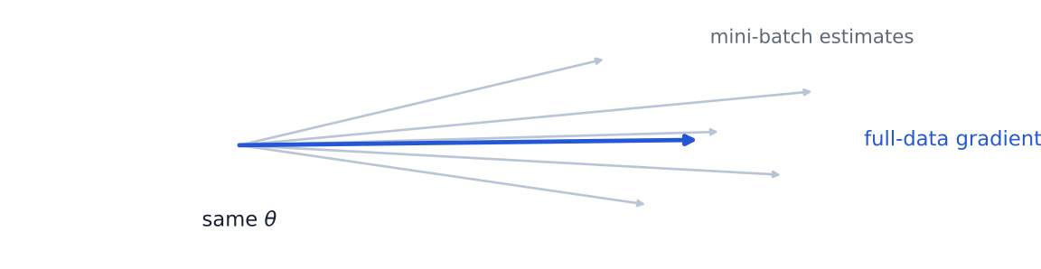
As Figure 14 suggests, successive mini-batches generally produce different directions because they contain different examples. Larger batches often reduce this sampling variability but require more computation and memory per update; smaller batches provide more frequent, noisier updates. Neither choice is universally superior.

An update step consumes one batch and performs one parameter update. An epoch is one pass through the available training examples, usually divided into many steps. Shuffling the training order between epochs helps prevent a fixed ordering from repeatedly producing systematically structured batches. It does not turn validation or test examples into training data.

The loss reduction controls gradient scale. Replacing the mean above with a sum multiplies the batch gradient by \(|\mathcal B_t|\) for the same examples. This changes the effective update scale unless the learning rate or another part of the procedure compensates. As established in the matrix-backpropagation section, the backward rules do not add a hidden factor: they differentiate the scalar loss they receive.

Learning rate and optimizer state

The learning rate \(\eta\) determines how strongly an update reacts to the optimizer’s proposed direction. If it is too small, reliable gradients can still yield impractically slow progress. If it is too large, updates can overshoot useful regions, oscillate, or drive the loss to non-finite values.

Figure 15: On the same schematic loss contours, a small learning rate barely moves, a useful scale approaches the low-loss region, and a large scale overshoots and oscillates.

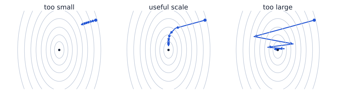
Figure 15 is deliberately schematic: no single numerical threshold separates the three regimes. The useful scale depends on the objective, parameterization, batch size, gradient scale, optimizer, and stage of training.

The gradient and the optimizer’s state are also different objects. Plain stochastic gradient descent without momentum can use the current gradient directly. Momentum maintains a running combination of present and past gradients. Adaptive optimizers such as Adam additionally maintain running statistics that rescale coordinates. These stored quantities persist across update steps; they are not produced anew by the current backward pass. Adam still needs a learning rate, and choosing it does not guarantee either successful optimization or generalization (PyTorch contributors, n.d.-i).

AdamW adds a separate shrinkage operation to Adam’s update. This decoupled weight decay is not the same algorithmic operation as inserting an L2 penalty—a squared-weight term—into the loss and then passing the resulting gradient through Adam’s adaptive transformation (Loshchilov and Hutter 2019). Both may discourage large weights, but the location of the operation in the training process differs.

Initialization controls signal scale

Before the first update, initialization determines the network’s forward values and the local derivatives available to the reverse pass. Setting every hidden unit to identical incoming weights and biases creates a symmetry: those units produce the same activation and receive the same gradient, so ordinary gradient updates do not make them learn different features. Random initialization breaks that symmetry.

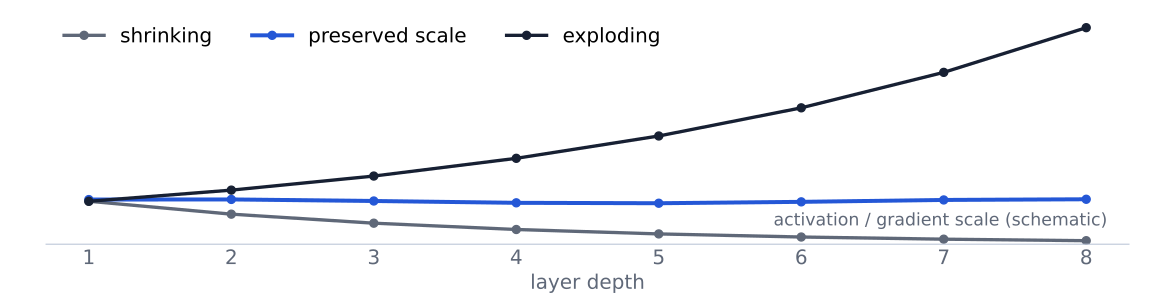
Randomness alone is not enough. If the initial weight scale is too small, activations and gradients can shrink across many layers. If it is too large, they can grow rapidly or push saturating activations into regions with weak derivatives. The aim is not to make every value identical across depth, but to keep useful signal scales from collapsing or exploding immediately.

Figure 16: Across increasing depth, poor initialization scales can make activations or gradients shrink toward zero or grow rapidly, while a suitable scale keeps them in a usable range.

Xavier or Glorot initialization chooses a variance based on both input and output fan sizes; in its common normal form, the variance is approximately

\[ \operatorname{Var}(W_{jk}) \approx \frac{2}{\operatorname{fan}_{\mathrm{in}}+\operatorname{fan}_{\mathrm{out}}}. \]

It was motivated by preserving useful activation and gradient variance under simplifying assumptions (Glorot and Bengio 2010). He or Kaiming initialization accounts for the fact that a ReLU blocks roughly part of a symmetric signal; its common fan-in normal form uses

\[ \operatorname{Var}(W_{jk}) \approx \frac{2}{\operatorname{fan}_{\mathrm{in}}}. \]

It is therefore a common choice for ReLU networks (He et al. 2015). PyTorch exposes Xavier and Kaiming variants with explicit gain, mode, nonlinearity, and fan conventions (PyTorch contributors, n.d.-h). These formulas are heuristics derived under distributional and independence approximations. They do not guarantee stable training, and their assumptions become less accurate as architecture, normalization, data distribution, or activation behavior changes. Figure 16 should therefore be read as the mechanism they try to control, not as a promise about every network.

Optimization is not generalization

Three data roles, three different questions

The 241-point curve fit in the companion tutorial shows that a nonlinear network can reduce loss and arrange ReLU bends around the observed training points. It demonstrates optimization and representation capacity on those points. Because that experiment does not establish performance on separate examples, it is not evidence that the fitted curve generalizes.

The distinction requires three data roles:

Data split	Primary role	Appropriate use
Training	Fit model parameters.	Supply the mini-batches used by the optimizer.
Validation	Compare development choices.	Select hyperparameters, architectures, checkpoints, or an early-stopping time.
Test	Estimate final performance after development choices are fixed.	Perform a final evaluation, not routine tuning.

A decreasing training loss answers a narrow but important question: the chosen optimizer is reducing the training objective for the current model and data. It does not establish that the model learned a relationship that transfers to new cases. Validation evidence supplies a provisional answer during development. The test set supplies the final held-out check. Repeatedly consulting test performance while changing the model turns the test set into part of the development process and weakens its claim to be an independent final assessment.

Reading training and validation curves together

Training and validation losses are most informative as a pair. Several qualitative patterns recur:

• If both decrease, optimization is improving the training fit and validation evidence is improving as well.
• If training loss continues downward while validation loss rises, the widening gap is evidence that later updates improve the training objective without improving the selected validation criterion.
• If both remain poor, the model may be underfitting, optimization may be ineffective, or the data and objective may be inadequate; the curves alone do not identify which cause is responsible.
• If validation loss is noisy, the split may be small or heterogeneous, or the evaluation metric may have high variability. A single favorable fluctuation should not be overinterpreted.

Figure 17: Training and validation loss initially fall together; later, training loss continues to improve while validation loss turns upward, creating a widening gap.

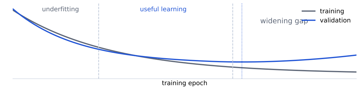
The dotted checkpoint in Figure 17 illustrates early stopping. A validation criterion selects a training time or saved checkpoint; the test set is not monitored to decide when to stop. Early stopping is therefore a model-selection procedure based on validation evidence, as well as a practical way to limit continued adaptation to the training sample.

A compact map of regularization

Regularization names interventions intended to improve performance beyond the fitted training examples, often by limiting, perturbing, or redirecting the learning process. The mechanisms do not all enter the mathematics at the same place:

• objective penalties add a term, such as an L1 or L2 penalty, to the scalar training objective;
• decoupled weight decay shrinks parameters as a separate part of the optimizer update;
• early stopping limits how long parameters adapt to the training data, using validation evidence to select a checkpoint;
• Dropout randomly masks selected activations during training;
• data augmentation constructs training examples through transformations intended to preserve task meaning;
• architectural or capacity constraints restrict the family of functions available to the learner.

Figure 18: Regularization mechanisms can act through the objective, the optimizer update, the network, or the data and duration of training.

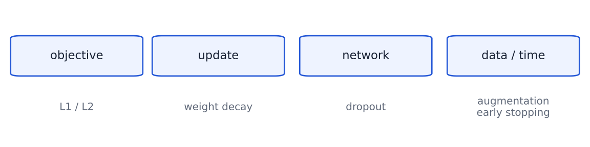
Figure 18 prevents a common conceptual collapse: regularization is not one extra term that always appears in the loss. The placement matters. An explicit penalty changes the gradient of the objective, whereas AdamW-style decay changes the update separately. Early stopping changes checkpoint selection. Augmentation changes the training examples encountered.

Dropout also returns us to the distinction among autograd controls. During training, a Dropout module randomly masks activations and rescales those retained; during evaluation, it behaves deterministically. Calling model.eval() selects the evaluation behavior. A no-grad context separately controls graph recording. Validation code normally needs both choices to be explicit.

This chapter does not yet develop the L2-as-Gaussian-prior or MAP interpretation, detailed Dropout theory, a full bias–variance framework, or a catalogue of tuning recipes. Those topics need more space and prerequisite structure than this training bridge can provide. We now have every component needed to reconstruct the complete learning argument.

Synthesis, exercises, and further reading

One connected learning system

The chapter began with a straight line that could not bend and ends with a procedure for learning, checking, and evaluating a nonlinear model. Its conceptual spine is

\[ \begin{aligned} \text{input} &\longrightarrow \text{learned representation}\\ &\longrightarrow \text{logits or prediction}\\ &\longrightarrow \text{loss}\\ &\longrightarrow \text{sensitivities}\\ &\longrightarrow \text{parameter update}\\ &\longrightarrow \text{validation evidence}. \end{aligned} \]

Each transition contributes something necessary, but none can establish the whole learning claim alone.

1. Input to learned representation. Affine transformations combine available features; nonlinear activations prevent a stack of layers from collapsing into one affine map. This enlarges the model family, but greater representation capacity does not ensure that optimization will find useful parameters.
2. Representation to logits or prediction. Forward propagation evaluates the current composition. Column-vector notation exposes one sample, while the batch-row convention exposes how the same operations run for many samples. A forward value is a model output, not yet evidence that the output is accurate or useful.
3. Output to loss. Task semantics determine the interpretation. Regression predictions can be compared directly with numerical targets; binary and multiclass classifiers produce logits that logits-based losses interpret stably. Softmax can express a multiclass probability vector, while the class target selects the observed component. A scalar loss measures the chosen discrepancy, but it does not explain which parameter caused it.
4. Loss to sensitivities. The chain rule assigns local sensitivities to every connected value. Scalar backpropagation multiplies derivatives along a path and adds contributions where paths meet. Matrix backpropagation performs the same work through vector–Jacobian products with shape-checked tensor operations. Autograd records and executes these local rules; it does not choose the model or update parameters.
5. Sensitivities to parameter update. An optimizer uses stored parameter gradients, a learning rate, and possibly state such as momentum or adaptive moments. backward() computes gradients; step() changes parameters. A valid local update can still be too large, too small, or poorly conditioned, and successful reduction of training loss still says nothing by itself about new data.
6. Updates to validation evidence. Repeated mini-batch updates fit the training objective. Validation data then inform checkpoint and hyperparameter choices without supplying optimizer updates. Only this separation lets us distinguish improved training fit from evidence of generalization; a reserved test set is used after development choices are fixed.

The result is one system rather than a list of neural-network terms. Representation determines what can be expressed. Forward propagation determines what the current parameters predict. The loss determines what discrepancy is optimized. Backpropagation and autograd determine the sensitivities. The optimizer determines how parameters move. Validation determines whether those choices remain promising away from the training batches.

Common confusions to keep separate

Distinction	Reliable test
Affine layer versus activation	nn.Linear computes an affine transformation; ReLU or another activation is a separate operation.
Logit versus probability	A logit is unconstrained. Sigmoid or Softmax maps logits to probabilities; logits-based losses receive logits directly.
Gradient versus update	A gradient is a local sensitivity stored by backpropagation. An optimizer uses it to construct an update.
Leaf versus non-leaf tensor	Leaves are graph endpoints such as ordinary trainable parameters; non-leaves are results of recorded operations. Both participate in differentiation, but non-leaf .grad is not retained by default.
detach() versus no_grad() versus eval()	detach() cuts one returned tensor from prior history; no_grad() disables recording for operations in a context; eval() changes modules with evaluation-specific behavior.
Training loss versus validation evidence	Training loss measures the objective being fitted. Validation results assess development choices on data not used for parameter updates.
L2 penalty versus decoupled weight decay	An L2 penalty contributes to the loss gradient. Decoupled weight decay acts separately in the optimizer update.

When debugging, naming the object in the left column is often more useful than asking whether “the network works.” It turns a vague failure into a check of representation, forward values, loss semantics, gradient flow, updates, or evaluation evidence.

Exercises

The exercises progress from algebra and forward calculations to gradient reasoning and training diagnosis. Unless a problem says otherwise, vectors for one sample are columns, batches store samples in rows, and class names in prose are one-based while PyTorch class-index targets are zero-based.

Exercise 1 — Three affine layers collapse

Let

\[ \mathbf h^{(1)}=\mathbf W^{(1)}\mathbf x+\mathbf b^{(1)}, \qquad \mathbf h^{(2)}=\mathbf W^{(2)}\mathbf h^{(1)}+\mathbf b^{(2)}, \]

\[ \mathbf y=\mathbf W^{(3)}\mathbf h^{(2)}+\mathbf b^{(3)}, \]

with widths \(d_0,d_1,d_2,d_3\). Prove by substitution that the complete mapping from \(\mathbf x\in\mathbb R^{d_0}\) to \(\mathbf y\in\mathbb R^{d_3}\) is affine. Give the equivalent weight matrix and bias vector, and verify their shapes. Explain precisely where this argument would fail if a ReLU were inserted after either of the first two layers.

Exercise 2 — Forward values and shapes

For one input, consider a \(2\to3\to1\) network:

\[ \mathbf x= \begin{bmatrix}1\\-2\end{bmatrix}, \quad \mathbf W^{(1)}= \begin{bmatrix} 1&0\\ -1&1\\ 0.5&-0.5 \end{bmatrix}, \quad \mathbf b^{(1)}= \begin{bmatrix}0\\1\\-0.5\end{bmatrix}. \]

The hidden activation is ReLU. The output layer is affine with

\[ \mathbf W^{(2)}= \begin{bmatrix}2&-1&0.5\end{bmatrix}, \qquad b^{(2)}=-1. \]

Compute \(\mathbf z^{(1)}\), \(\mathbf h^{(1)}\), and \(\hat y\). Annotate the shape of every input, parameter, and intermediate. Then suppose a batch matrix \(\mathbf X\) contains four samples in its rows. State the shapes of \(\mathbf X\), \(\mathbf Z^{(1)}\), \(\mathbf H^{(1)}\), and the final batch output, and write the batch equation for the first layer using PyTorch’s stored-weight orientation.

Exercise 3 — Confidence and cross-entropy

A three-class classifier observes class 3 in one-based naming. Its PyTorch class-index target is therefore 2, and its one-hot target is \([0,0,1]\). Compare two logit vectors:

\[ \mathbf z_{\mathrm{correct}}=[0,0,4], \qquad \mathbf z_{\mathrm{wrong}}=[4,0,0]. \]

For each vector, compute Softmax probabilities to at least four decimal places, identify the argmax class, and compute the observed-class cross-entropy. Explain why the two losses differ greatly even though the same three numerical logit values appear in both vectors. State exactly what target tensor would be passed to F.cross_entropy for a batch containing only this example.

Exercise 4 — Predict gradient signs first

Use

\[ z=wx+b, \qquad h=\operatorname{ReLU}(z), \qquad \hat y=ah+c, \qquad L=\frac12(\hat y-y)^2, \]

with

\[ x=2,\quad w=-1,\quad b=3,\quad a=-2,\quad c=4,\quad y=1. \]

Before calculating exact derivatives, predict the signs of \(\partial L/\partial a\), \(\partial L/\partial w\), and \(\partial L/\partial x\). Justify each sign by describing how a small positive change would affect the prediction and loss. Then perform the complete forward pass and calculate the gradients with respect to \(a,c,w,b,x\). Reconcile each exact result with the sign prediction.

Exercise 5 — From one weight entry to the matrix product

For one affine-plus-activation layer, suppose the activation derivative has already been applied and

\[ \mathbf H_{\mathrm{in}}= \begin{bmatrix} 1&2\\ -1&3 \end{bmatrix}, \qquad \mathbf G_Z= \begin{bmatrix} 2&-1\\ 4&0.5 \end{bmatrix}. \]

Here \(B=2\), \(d_{\mathrm{in}}=2\), and \(d_{\mathrm{out}}=2\). Using one-based mathematical indices, derive \(\partial L/\partial W_{12}\) directly as a sum over the two batch rows. Then compute the complete matrix \(\partial L/\partial\mathbf W=\mathbf G_Z^\top\mathbf H_{\mathrm{in}}\) and the bias gradient. Verify every shape and explain why reversing the matrix-product order is incorrect.

Exercise 6 — Two meanings of “accumulate”

Let a scalar parameter start at \(p=0\), with learning rate \(\eta=0.1\), and define two losses

\[ L_1(p)=\frac12(p-1)^2, \qquad L_2(p)=\frac12(p-3)^2. \]

Analyze two distinct scenarios.

1. Two backward calls, one update: evaluate both losses at \(p=0\), call backward() on each without clearing .grad, and call step() only after both backward calls. What gradient is stored, and what value of \(p\) results? Is this the gradient of a sum or a mean?
2. Two updates, stale gradient: evaluate \(L_1\), call backward() and step(), then evaluate \(L_2\) at the new parameter value but omit zero_grad() before the second backward() and step(). Compute the resulting \(p\). Compare it with the result when the gradient is correctly cleared before the second backward call.

For each scenario, say whether gradient accumulation is deliberate or accidental. Keep separate the addition across backward calls from the chain-rule addition of multiple paths within one graph.

Exercise 7 — Diagnose curves before prescribing a remedy

For each qualitative pattern below, give (i) at least two plausible interpretations and (ii) one next diagnostic that would help distinguish them. Do not prescribe a single automatic remedy from the curves alone.

1. Training and validation loss both decrease steadily.
2. Training loss decreases while validation loss reaches a minimum and then rises.
3. Training and validation loss remain high and nearly flat.
4. Training loss is smooth, while validation loss varies sharply from one evaluation to the next.

For pattern 2, explain how early stopping should select a checkpoint and why the test set must not choose the stopping time. For pattern 4, include the possible role of validation-set size or heterogeneity.

Exercise 8 — A central finite-difference check

Use the scalar network and numerical values from Exercise 4. Treat every quantity except \(w\) as fixed and define \(L(w)\) through the complete forward calculation. With \(\varepsilon=10^{-5}\), estimate

\[ \frac{\partial L}{\partial w} \approx \frac{L(w+\varepsilon)-L(w-\varepsilon)}{2\varepsilon}. \]

Compare the estimate with the analytic gradient from Exercise 4. Describe a reasonable absolute or relative tolerance for a float64 check, and explain why an extremely small \(\varepsilon\), an excessively large \(\varepsilon\), or a perturbation that crosses a ReLU breakpoint can make the comparison misleading.

Further reading

The following sources extend particular parts of the chapter without being prerequisites for it:

• Chapter 6 of Deep Learning gives a broader treatment of feedforward networks, output units, hidden units, and backpropagation (Goodfellow et al. 2016).
• Baydin and colleagues place reverse-mode differentiation within the wider family of automatic-differentiation methods and distinguish it from symbolic and numerical differentiation (Baydin et al. 2018).
• Rumelhart, Hinton, and Williams provide a historically influential primary presentation of learning internal representations with backpropagation (Rumelhart et al. 1986).
• PyTorch’s autograd mechanics note documents the graph, gradient modes, and evaluation-mode distinctions used in this chapter (PyTorch contributors, n.d.-a).
• The Glorot and He papers develop the initialization arguments summarized in the training-process section (Glorot and Bengio 2010; He et al. 2015).

Looking ahead: convolutional neural networks

The next curricular chapter introduces convolutional neural networks. CNNs retain the same machinery developed here: a forward pass produces logits or predictions, a loss evaluates them, reverse-mode differentiation computes sensitivities, an optimizer updates parameters, and validation evidence evaluates development choices. What changes is the structure of the learned affine transformation. Local connections, shared parameters, and spatial organization encode assumptions suited to grid-like data. Those ideas deserve their own derivation; the present chapter supplies the learning process on which they build.

Baydin, Atilim Gunes, Barak A. Pearlmutter, Alexey Andreyevich Radul, and Jeffrey Mark Siskind. 2018. “Automatic Differentiation in Machine Learning: A Survey.” Journal of Machine Learning Research 18 (153): 1–43. https://www.jmlr.org/papers/v18/17-468.html.

Glorot, Xavier, and Yoshua Bengio. 2010. “Understanding the Difficulty of Training Deep Feedforward Neural Networks.” Proceedings of the Thirteenth International Conference on Artificial Intelligence and Statistics, Proceedings of machine learning research, vol. 9: 249–56. https://proceedings.mlr.press/v9/glorot10a.html.

Goodfellow, Ian, Yoshua Bengio, and Aaron Courville. 2016. Deep Learning. MIT Press. https://www.deeplearningbook.org/.

He, Kaiming, Xiangyu Zhang, Shaoqing Ren, and Jian Sun. 2015. “Delving Deep into Rectifiers: Surpassing Human-Level Performance on ImageNet Classification.” Proceedings of the IEEE International Conference on Computer Vision, 1026–34. https://openaccess.thecvf.com/content_iccv_2015/html/He_Delving_Deep_into_ICCV_2015_paper.html.

Loshchilov, Ilya, and Frank Hutter. 2019. “Decoupled Weight Decay Regularization.” International Conference on Learning Representations. https://arxiv.org/abs/1711.05101.

PyTorch contributors. n.d.-a. “Autograd Mechanics.” Accessed September 24, 2026. https://docs.pytorch.org/docs/stable/notes/autograd.html.

PyTorch contributors. n.d.-b. “BCEWithLogitsLoss — PyTorch Documentation.” Accessed September 27, 2026. https://docs.pytorch.org/docs/stable/generated/torch.nn.BCEWithLogitsLoss.html.

PyTorch contributors. n.d.-c. “CrossEntropyLoss — PyTorch Documentation.” Accessed September 24, 2026. https://docs.pytorch.org/docs/stable/generated/torch.nn.CrossEntropyLoss.html.

PyTorch contributors. n.d.-d. “Linear — PyTorch Documentation.” Accessed September 27, 2026. https://docs.pytorch.org/docs/stable/generated/torch.nn.Linear.html.

PyTorch contributors. n.d.-e. “Optimizer.zero_grad — PyTorch Documentation.” Accessed September 24, 2026. https://docs.pytorch.org/docs/stable/generated/torch.optim.Optimizer.zero_grad.html.

PyTorch contributors. n.d.-f. “Tensor.detach — PyTorch Documentation.” Accessed September 24, 2026. https://docs.pytorch.org/docs/stable/generated/torch.Tensor.detach.html.

PyTorch contributors. n.d.-g. “Tensor.retain_grad — PyTorch Documentation.” Accessed September 24, 2026. https://docs.pytorch.org/docs/stable/generated/torch.Tensor.retain_grad.html.

PyTorch contributors. n.d.-h. “torch.nn.init — PyTorch Documentation.” Accessed September 24, 2026. https://docs.pytorch.org/docs/stable/nn.init.html.

PyTorch contributors. n.d.-i. “torch.optim — PyTorch Documentation.” Accessed September 24, 2026. https://docs.pytorch.org/docs/stable/optim.html.

Rumelhart, David E., Geoffrey E. Hinton, and Ronald J. Williams. 1986. “Learning Representations by Back-Propagating Errors.” Nature 323: 533–36. https://doi.org/10.1038/323533a0.