← Course homeAll chapters

Week 05 · Visual Representation Learning: Local Patterns, Shared Weights, and Convolutional Networks

A vertical edge can occur near the left border of an image, near the center, or near the right border. Its location changes, but the local relationship between darker and brighter pixels can remain the same. A useful visual model should be able to reuse that relationship rather than learn it independently at every possible location.

Week 04 supplied the machinery for learning representations: affine transformations, nonlinear activations, a loss, backpropagation, and parameter updates. Convolutional neural networks (CNNs) retain that machinery while imposing structure on the affine transformations. Each early output uses a local neighborhood, and the same parameters act at many spatial positions. These choices express assumptions about the input: nearby measurements matter together, and similar local patterns recur.

We will first make those assumptions precise through images and small numerical calculations. We will then derive how shared parameters receive gradients from all their uses. We will develop spatial geometry, deeper architectures, normalization, and transfer learning, then use a controlled signal-classification experiment to judge whether this structure helps a particular task.

English Русский

Learning outcomes

After reading the chapter, you should be able to:

1. explain and compute convolutional representations using explicit tensor axes, local connectivity, and shared parameters;
2. derive shared-weight gradients and account for convolutional shapes and parameter counts;
3. reason about padding, stride, pooling, receptive fields, and translation behavior;
4. explain residual learning and normalization, including their gradients, axes, and state;
5. choose and check augmentation, frozen-feature transfer, and fine-tuning policies; and
6. interpret a controlled model comparison, distinguishing validation decisions and supported test conclusions from broader claims.

Prerequisites and companion materials

We assume matrix multiplication, scalar derivatives, and the Week 04 account of forward propagation and the chain rule. In particular, the Week 04 chapter explains why derivatives multiply along a path and add where paths meet. No image-processing background is required here.

The Week 05 lecture provides the visual teaching sequence. The Convolutions tutorial exposes the calculations and checks them against PyTorch. This chapter reuses selected figures and numerical examples while developing the reasoning in prose. The tutorial’s progression from a hand-calculated response to a scanned map acknowledges fastai’s convolution chapter; the course examples and figures used here are independently constructed.

Why image structure changes the model

What did Hubel and Wiesel measure?

A visual neuron need not respond equally to everything in a scene. In their 1959 study, David Hubel and Torsten Wiesel recorded individual cells in the visual cortex of lightly anaesthetized cats while presenting light patterns. Changing the stimulus position and orientation changed the responses of some cells (Hubel and Wiesel 1959).

Figure 1: Schematic of the historical visual-selectivity experiment. The drawing, spike trains, and tuning curve illustrate the idea; they are not measurements reproduced from the paper. Instructor-supplied lecture illustration, shown unchanged.

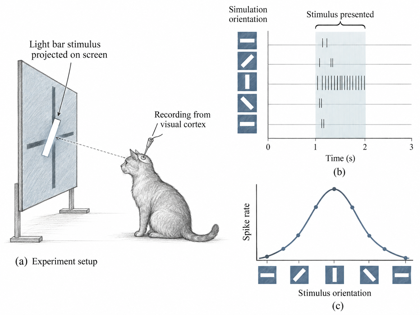
Two questions are different. Where can a stimulus influence this cell? That region is its receptive field. Which pattern evokes a strong response within that region? This is selectivity: a bar at one orientation can produce a stronger response than the same bar turned another way.

This suggests a useful engineering question: can we build a computation that responds to a particular relationship among nearby pixels? A small weighted window provides one simple answer. Reusing exactly the same weights at every location is a further design choice. The biological experiment motivates local selectivity; it does not establish the CNN’s exact parameter-sharing rule.

From a selective response to an engineered detector

Imagine comparing the brightness on the right side of a small patch with the brightness on its left. Subtract the left values and add the right values. A uniform patch cancels; a dark-to-bright boundary gives a positive response; reversing the boundary changes the sign. We have constructed a local question without training a model.

Alternatively, give all pixels equal positive weights that sum to one. Now the answer is the local mean. The pixels are the same; choosing different coefficients changes what we measure. These fixed, hand-designed filters let us understand the operation before learning its coefficients from data.

Channels describe what; spatial axes describe where

A grayscale image contains one intensity measurement at each position. An RGB image contains three measurements at each position: red, green, and blue. These are channels of one image. A batch contains several images, each with its own channels and spatial coordinates.

We use the batch-first image layout

\[ \mathbf X\in\mathbb R^{B\times C_{\mathrm{in}}\times H\times W}. \]

\(\mathbb R\) denotes real numbers; the expression says that \(\mathbf X\) is a real-valued tensor with the displayed axis sizes. Bold symbols denote whole vectors, matrices, or tensors, while indexed plain symbols denote individual entries. Here \(B\) is the number of examples, \(C_{\mathrm{in}}\) the number of input channels, and \(H,W\) the height and width. Plain \(W\) denotes a spatial width; bold \(\mathbf W\) denotes a parameter tensor. When no input/output distinction is needed, \(C\) denotes the channel count. An image display library often places channels last, giving \((H,W,C)\) for one RGB image. PyTorch’s convolutional layout places channels before the spatial axes, giving \((C,H,W)\) for one image and \((B,C,H,W)\) for a batch. The values retain their meaning when axes are reordered.

Figure 2: One image can be viewed as a composite or as separate channel planes. The outlined pixel has the same spatial coordinates in every plane; the layout changes where its channel index is written. Course-generated tensor illustration from the Week 05 tutorial.

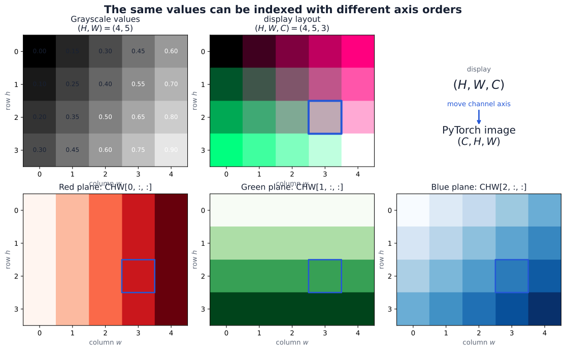
Display libraries often store one image as \((H,W,C)\), whereas the convolution here uses \((B,C,H,W)\). Moving an axis requires a permutation; reshaping alone does not generally perform that conversion. The tutorial’s image-tensor scene follows one pixel through the conversion.

Locality and sharing constrain different things

A dense layer can give each output an independently adjustable coefficient for every input value. Flattening an image makes such a layer possible, but the architecture then supplies no special treatment of neighboring pixels. Spatial relationships may still be learned from data; they are not built into that connectivity.

Locality restricts one output to a small spatial neighborhood. Parameter sharing reuses one set of local coefficients at many neighborhoods. These constraints are separate: a locally connected layer could assign different coefficients to different positions. A convolution combines locality with sharing, asking the same learned local question wherever its window is evaluated.

From one local calculation to a convolutional layer

A fixed kernel defines a signed local response

Begin with a single image channel and one \(3\times3\) window. A kernel assigns a coefficient to each relative position inside the window. Multiplying matching entries and summing the products produces one scalar response.

The local mean is also called a blur. An edge filter instead assigns opposite signs to opposite sides of a window. Before reading the matrices, predict which of these operations should return zero on a constant patch. The three kernels are:

\[ \begin{aligned} \mathbf W_{\mathrm{mean}} &=\frac{1}{9} \begin{bmatrix}1&1&1\\1&1&1\\1&1&1\end{bmatrix},\\[3pt] \mathbf W_{\mathrm{horizontal}} &=\begin{bmatrix}-1&-1&-1\\0&0&0\\1&1&1\end{bmatrix},\\[3pt] \mathbf W_{\mathrm{vertical}} &=\begin{bmatrix}-1&0&1\\-1&0&1\\-1&0&1\end{bmatrix}. \end{aligned} \]

The first computes a local mean. The second compares the bottom row with the top row, while the third compares the right column with the left column. For the contrast kernels, sign records orientation: a dark-to-bright transition moving downward or rightward gives a positive response under the displayed convention. Reversing that transition reverses the sign.

For the tutorial’s selected patch \(\mathbf P\), whose entries are the pixel values in one window,

\[ \mathbf P= \begin{bmatrix} 0&0&0\\ 1&1&1\\ 1&1&1 \end{bmatrix}, \]

write \(R_{\mathrm{mean}},R_{\mathrm{horizontal}},R_{\mathrm{vertical}}\) for the scalar responses of the three named kernels:

\[ \begin{aligned} R_{\mathrm{mean}}&=6/9=2/3,\\ R_{\mathrm{horizontal}}&=(-1)(0+0+0)+(1)(1+1+1)=3,\\ R_{\mathrm{vertical}}&=(0-0)+(1-1)+(1-1)=0. \end{aligned} \]

The zero vertical response means that left-right contributions cancel in this patch. It does not mean that the patch is empty. Different kernels measure different relationships in the same values.

Scanning turns local responses into maps

Let \(a,c\) index an output row and column, and let \(u,v\) index relative row and column offsets within the kernel. \(k_H,k_W\) are kernel height and width, \(W_{u,v}\) is a kernel coefficient, and \(X_{a+u,c+v}\) is the paired image value. All these coordinate indices start at zero. With stride 1, no padding, and no bias, the response \(R_{a,c}\) is

\[ R_{a,c} =\sum_{u=0}^{k_H-1}\sum_{v=0}^{k_W-1} W_{u,v}X_{a+u,c+v}. \]

The output coordinate identifies the window’s top-left corner in this unpadded input. Scanning a \(3\times3\) window across the \(7\times7\) toy image permits starts 0 through 4 on each axis. Each kernel therefore produces a \(5\times5\) response map. The selected patch above starts at row 1, column 2, so its three responses occupy location \((1,2)\) in the corresponding maps.

Figure 3: The same selected window answers three local questions. Each kernel is reused across the complete image, and the highlighted response cell records the calculation for that window. Course-generated, checked toy example from the Week 05 tutorial.

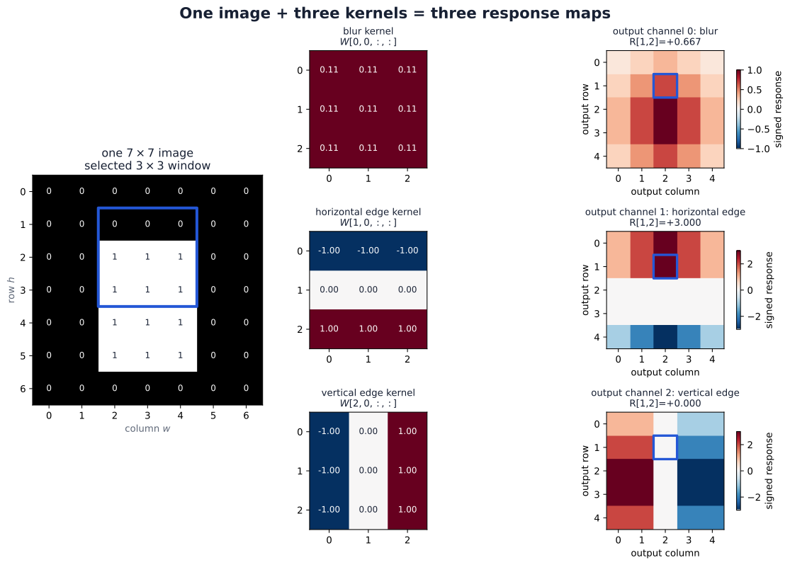
This repeated local calculation is the core of convolution: a kernel holds the local weights, and its scanned answers form a response map. The coefficients remain unchanged as the window moves. The map records how each neighborhood responds to one fixed question. These values are signed measurements; they need not lie between zero and one, and a display color scale does not change their numerical meaning.

In the mathematical convention for convolution, kernel coordinates are reversed. The operation displayed here uses the coefficients in their stored order and is called cross-correlation. PyTorch and the deep-learning materials call this operation convolution; we follow that terminology while keeping the unflipped convention explicit. See the PyTorch Conv2d definition.

One output filter combines all input channels

A color image gives us three aligned measurements at every pixel: red, green, and blue. Select one spatial window. It contains a red patch, a green patch, and a blue patch at the same coordinates. How can these become one response?

A complete filter has one kernel slice for each input channel. Pair the red patch with the red slice, multiply matching entries, and sum. Do the same for green and blue. Add the three contributions and one bias to obtain a single preactivation. The slices can have different values: the filter can compare colors as well as spatial positions.

Figure 4: One RGB patch is combined with one complete filter to produce one response, then a bias and ReLU produce one activation-map entry. Only the first row of the instructor-supplied illustration is shown.

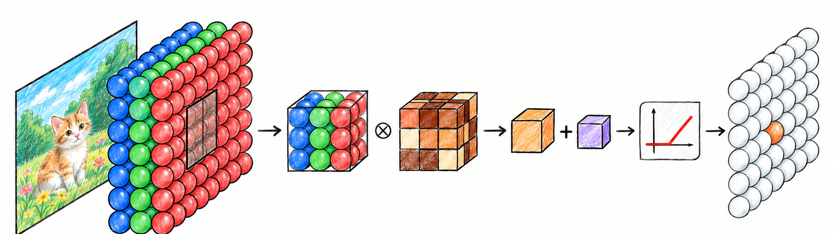
Read the illustration from left to right. The multiplication symbol represents matching-entry products and their sum over the whole patch, not three separate output maps. The small cube after it represents one scalar. Adding the bias completes the affine operation; the red graph is ReLU, which clips negative preactivations to zero. Moving the complete filter over height and width fills one map. It does not slide along the channel axis.

For a \(3\times3\) RGB window, one filter contains three slices of nine coefficients each. A second filter owns another complete set of slices and its own bias. Scanning both filters gives two output maps, with weight shape \((2,3,3,3)\) and parameter count

\[ 2\cdot3\cdot3\cdot3+2=56. \]

The first axis counts output filters, the second counts input channels, and the final two count spatial offsets. The three occurrences of 3 happen to be equal; they name different things. The tutorial’s color example works through two hand-designed filters on the Chelsea photograph: luminance vertical contrast and warm-versus-blue local mean.

NotePause and predict: channels and filters

An RGB convolution has four output filters. Does each filter see only one color, and how many output maps will it produce?

Reveal the explanation

Each ordinary filter combines all three input channels using three kernel slices. Each complete filter produces one map, so four filters produce four output maps. Input channels and output filters count different things.

From colors to learned feature maps

After the first layer, input channels are no longer necessarily red, green, and blue. They are maps produced by the previous layer: different learned measurements at each location. A later filter can combine a response in one channel with nearby responses in other channels. The computation is unchanged; the meaning of its inputs has changed.

Suppose a hidden layer receives eight input maps and should produce sixteen output maps. Each of its sixteen filters contains eight spatial slices. Input channel count says how many measurements a filter combines; output channel count says how many different filters we apply. Neither count is the number of classes. Feature map is a common broad name for a channel’s map. Here we use response map for a fixed filter’s output and activation map for a learned representation after an activation.

The general affine layer and its shapes

We can now assemble the indexed operation. The function \(\phi\) is an elementwise activation applied after the affine calculation. For this derivation, suppress the layer superscript: \(\mathbf h\) is the input representation, \(\mathbf z\) the output preactivation, and \(\mathbf W,\mathbf b\) the layer parameters. Let \(\widetilde{\mathbf h}\) denote the input after padding. With symmetric zero padding of width \(p_H,p_W\), original coordinate \((q,t)\) appears at padded coordinate \((q+p_H,t+p_W)\), and locations outside the original image are zero.

For the ordinary ungrouped operation with adjacent kernel entries (groups=1, dilation=1),

\[ \begin{aligned} z_{n,o,a,c} &=b_o+ \sum_{i=0}^{C_{\mathrm{in}}-1} \sum_{u=0}^{k_H-1} \sum_{v=0}^{k_W-1} W_{o,i,u,v}\, \widetilde h_{n,i,a s_H+u,c s_W+v},\\ h^{\mathrm{out}}_{n,o,a,c} &=\phi(z_{n,o,a,c}). \end{aligned} \]

Here \(n\) selects an example’s row within the batch, from 0 through \(B-1\); \(o\) selects an output filter; \(i\) selects an input channel; and \(s_H,s_W\) are the strides between evaluated window starts. The symbols \(a,c\) identify spatial output coordinates; the bias \(b_o\) is a scalar attached to output channel \(o\). The three sums combine all input channels and all positions in one local window. The same \(W_{o,i,u,v}\) and \(b_o\) are used for every example and every evaluated spatial position.

Here \(C_{\mathrm{out}}\) is the number of output filters, and \(H_{\mathrm{out}},W_{\mathrm{out}}\) are the output height and width. The superscript \(\mathrm{out}\) labels the output representation. The corresponding shapes are

\[ \begin{aligned} \mathbf h&\in\mathbb R^{B\times C_{\mathrm{in}}\times H\times W},\\ \mathbf W&\in\mathbb R^{C_{\mathrm{out}}\times C_{\mathrm{in}}\times k_H\times k_W},\\ \mathbf b&\in\mathbb R^{C_{\mathrm{out}}},\\ \mathbf z,\mathbf h^{\mathrm{out}} &\in\mathbb R^{B\times C_{\mathrm{out}}\times H_{\mathrm{out}}\times W_{\mathrm{out}}}. \end{aligned} \]

This also explains the parameter count:

\[ N_{\mathrm{parameters}} =C_{\mathrm{out}}C_{\mathrm{in}}k_Hk_W+C_{\mathrm{out}} \]

when biases are included. Batch size and output spatial dimensions do not appear in it. Increasing the number of evaluated windows increases the number of applications of each parameter rather than adding independently adjustable parameters.

The distinction between \(\mathbf z\) and \(\mathbf h^{\mathrm{out}}\) matters: the signed evidence before ReLU differs from the representation after negative entries have been removed.

Why sharing saves parameters

Consider a grayscale \(28\times28\) image and an output of eight \(28\times28\) maps. A dense layer has 784 inputs and \(8\cdot28\cdot28=6272\) outputs. With one bias for each output, its parameter count is

\[ 784\cdot6272+6272=4{,}923{,}520. \]

An ordinary convolution producing the same output shape with eight \(3\times3\) filters, stride 1, and one pixel of zero padding on every side has

\[ 8\cdot1\cdot3\cdot3+8=80 \]

parameters. Padding permits the windows near the image border; its geometry is developed in the spatial-geometry section. The eight biases are shared spatially, just as the filter weights are.

The two layers have equal input and output dimensions but different function classes. The dense layer may distinguish the same pattern at different locations through unrelated coefficients. The convolution requires the local rule to be reused. The parameter saving follows from this restriction; it does not establish predictive accuracy or wall-clock speed.

That restriction is an inductive bias: a preference encoded in the model before seeing the training examples. It is useful when nearby measurements interact and similar patterns recur across positions. It can be inappropriate when absolute position changes a pattern’s meaning or when the ordering of features is arbitrary. We must eventually test the architectural assumption against validation evidence.

Reading the PyTorch operation as mathematics

In the tutorial’s three-kernel grayscale calculation, the input shape is \((1,1,7,7)\), the stacked weights have shape \((3,1,3,3)\), and the result has shape \((1,3,5,5)\):

import torch.nn.functional as F

# image_hw: (7, 7); kernel_bank: (3, 3, 3)
image_batch = image_hw[None, None, :, :]
weights = kernel_bank[:, None, :, :]
responses = F.conv2d(image_batch, weights, bias=None)
assert responses.shape == (1, 3, 5, 5)

This snippet supplies existing fixed weights to a functional operation. A trainable nn.Conv2d module instead owns its weight and optional bias parameters. For example, nn.Conv2d(3, 2, kernel_size=3) stores the 56 parameters counted in the RGB example. It can learn different coefficients through backpropagation; an activation remains a separate operation. The API’s shape and operation conventions are documented in PyTorch Conv2d.

Important

An output channel is one complete filter’s response across positions. Its index does not automatically name a color or a class. A ten-class classifier need not have ten channels in every hidden layer; we reserve \(K\) for class count and \(C\) for channels.

Learning shared parameters

The forward calculation is now familiar. Training changes the coefficients so that the resulting maps help the task. One shared update changes the local question everywhere it is asked.

The learning loop remains familiar

A model \(f_\theta\) maps an input to a prediction, with \(\theta\) collecting its trainable parameters. For a mini-batch \(\mathcal B\) containing \(B\) examples, write the objective as

\[ \mathcal L_{\mathcal B} =\frac{1}{B}\sum_{n\in\mathcal B}\ell_n, \qquad \ell_n=L\!\left(f_\theta(\mathbf x_n),y_n\right). \]

Here \(n\) indexes an example, \(\mathbf x_n\) is its input, and \(y_n\) its target; \(\sum\) adds the example losses over the batch. This refines Week 04’s generic loss notation \(L\): \(\ell_n\) is one example’s loss, and \(\mathcal L_{\mathcal B}\) is the mean objective used for the batch update. The forward pass, loss calculation, backward pass, and optimizer retain their earlier jobs. A convolution changes how the model constructs its representations.

For layer \(\ell\), keep the same distinction between preactivation and representation:

\[ \begin{aligned} \mathbf z^{(\ell)} &=\operatorname{Conv}\!\left( \mathbf h^{(\ell-1)};\mathbf W^{(\ell)},\mathbf b^{(\ell)} \right),\\ \mathbf h^{(\ell)}&=\phi\!\left(\mathbf z^{(\ell)}\right), \qquad \mathbf h^{(0)}=\mathbf X. \end{aligned} \]

Here \(\ell\) is the layer index, \(\mathbf W^{(\ell)}\) and \(\mathbf b^{(\ell)}\) are its weights and biases, \(\mathbf z^{(\ell)}\) contains preactivations, and \(\mathbf h^{(\ell)}\) is the learned representation after the activation function \(\phi\). The input representation \(\mathbf h^{(0)}\) is the input tensor \(\mathbf X\); \(\operatorname{Conv}\) denotes convolution with the specified parameters. Parenthesized superscripts label layers, not powers.

The convolution with a bias is affine in its input for fixed parameters. The activation supplies the nonlinearity. Learning adjusts the entries of \(\mathbf W^{(\ell)}\) and \(\mathbf b^{(\ell)}\) through the same objective and chain rule used for a dense network.

The same two weights at every position

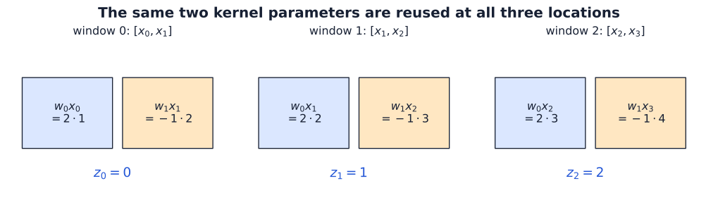
For the simplest trainable example, use one one-dimensional input channel,

\[ \mathbf x=\begin{bmatrix}1&2&3&4\end{bmatrix}^{\!\top}, \qquad \mathbf w=\begin{bmatrix}w_0&w_1\end{bmatrix}^{\!\top} =\begin{bmatrix}2&-1\end{bmatrix}^{\!\top}. \]

Here \(x_t\) denotes input position \(t\), and \(w_0,w_1\) are the two shared kernel coefficients. The superscript \(\top\) transposes a row into a column vector; it is not a time index. With stride 1, no padding, bias, or activation, the three preactivations \(z_t\) are

\[ \begin{aligned} z_0&=w_0x_0+w_1x_1=2(1)-1(2)=0,\\ z_1&=w_0x_1+w_1x_2=2(2)-1(3)=1,\\ z_2&=w_0x_2+w_1x_3=2(3)-1(4)=2. \end{aligned} \]

Each line refers to the same two parameters. Sharing is an identity constraint, not a coincidence in the initial values: updating \(w_0\) changes its contribution at every position.

Figure 5: Every overlapping window uses the same two parameter identities. Colors distinguish the reused parameters, rather than independent weights or numerical signs. Checked width-2 example from the Week 05 tutorial.

The chain rule sums contributions from every use

To expose the derivatives, define the illustrative scalar

\[ J=z_0+z_1+z_2. \]

Here \(J\) names this scalar probe, and \(t\) indexes an output position. The notation \(\partial J/\partial z_t\) means the derivative of \(J\) with respect to that output, holding other independent quantities fixed. This is a probe of the computation, not a predictive training loss. Since each \(\partial J/\partial z_t=1\), the chain rule gives

\[ \begin{aligned} \frac{\partial J}{\partial w_0} &=\sum_{t=0}^{2} \frac{\partial J}{\partial z_t} \frac{\partial z_t}{\partial w_0} =x_0+x_1+x_2=6,\\ \frac{\partial J}{\partial w_1} &=\sum_{t=0}^{2} \frac{\partial J}{\partial z_t} \frac{\partial z_t}{\partial w_1} =x_1+x_2+x_3=9. \end{aligned} \]

This is the Week 04 branch-addition rule applied to repeated uses of a parameter. Each path contributes a downstream sensitivity multiplied by its local derivative, and all paths to the shared parameter contribute to one gradient entry.

import torch
import torch.nn.functional as F

x = torch.tensor([1., 2., 3., 4.])
w = torch.tensor([2., -1.], requires_grad=True)
z = F.conv1d(x.reshape(1, 1, 4), w.reshape(1, 1, 2))
J = z.sum()
J.backward()
torch.testing.assert_close(z.flatten(), torch.tensor([0., 1., 2.]))
torch.testing.assert_close(w.grad, torch.tensor([6., 9.]))

For a general scalar objective \(\mathcal L\), define \(\delta_t=\partial\mathcal L/\partial z_t\), the sensitivity of the objective to output \(z_t\). The same derivation gives

\[ \frac{\partial\mathcal L}{\partial w_0} =\delta_0x_0+\delta_1x_1+\delta_2x_2, \qquad \frac{\partial\mathcal L}{\partial w_1} =\delta_0x_1+\delta_1x_2+\delta_2x_3. \]

Unlike the simple \(J\) example, sensitivities can differ in magnitude and sign. Some uses can reinforce each other while others cancel. Sharing combines their evidence into a single adjustment rather than allowing each position to choose its own update.

NotePause and predict: one parameter, several uses

In the width-2 example, \(w_0\) appears at three positions. Does backpropagation produce three independently adjustable gradients for it, or one gradient? Explain before opening the answer.

Reveal the explanation

There is one stored parameter and one gradient entry. The three paths contribute to that entry through the chain rule. For the displayed probe \(J=z_0+z_1+z_2\), the contributions are \(1,2,3\), which sum to \(6\). Independently adjustable entries would remove the sharing constraint.

Optional view: a sparse matrix with tied entries

The same operation can be expressed as

\[ \mathbf z=A(\mathbf w)\mathbf x, \qquad A(\mathbf w)= \begin{bmatrix} w_0&w_1&0&0\\ 0&w_0&w_1&0\\ 0&0&w_0&w_1 \end{bmatrix}. \]

\(\mathbf z=(z_0,z_1,z_2)^\top\) collects the outputs, and \(A(\mathbf w)\) is the effective matrix determined by the compact kernel. Zeros express locality; repeated parameter labels express sharing. If the six nonzero entries were independent parameters, this would be a locally connected layer with a separate rule at each position. Tying the three occurrences of \(w_0\) together, and likewise those of \(w_1\), yields the convolution.

Figure 6: The expanded matrix exposes both constraints: zeros prevent distant connections, while repeated labels require the same coefficient at shifted positions. This is an analytical view of the operation; the module stores the compact kernel.

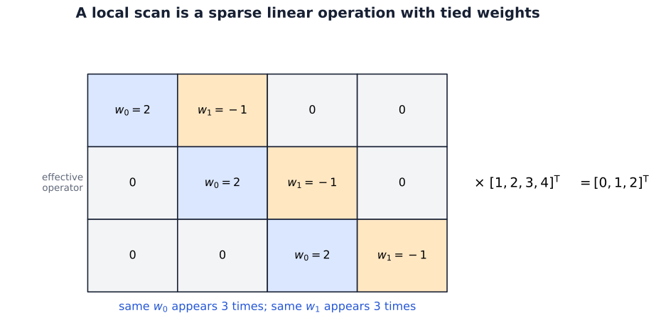
The map is linear in the input before a bias is added. Its coefficients depend on the parameters, so training can change the map while retaining its sparsity and tying pattern. There is no need to store the expanded matrix to evaluate it.

The gradient rule for an image batch

Return to the two-dimensional layer and define the preactivation sensitivity tensor

\[ \delta_{n,o,a,c} =\frac{\partial\mathcal L_{\mathcal B}}{\partial z_{n,o,a,c}}. \]

Its shape is the same as \(\mathbf z\). The prime in \(\phi'(z)\) below denotes the activation’s scalar derivative at \(z\). If an elementwise activation follows the convolution, the downstream representation gradient first passes through its local derivative:

\[ \delta_{n,o,a,c} =\frac{\partial\mathcal L_{\mathcal B}} {\partial h^{\mathrm{out}}_{n,o,a,c}} \,\phi'(z_{n,o,a,c}). \]

For one coefficient \(W_{o,i,u,v}\), the local derivative at a position using it is precisely the paired padded input value. Applying the chain rule to all its uses gives

\[ \frac{\partial\mathcal L_{\mathcal B}}{\partial W_{o,i,u,v}} =\sum_{n=0}^{B-1} \sum_{a=0}^{H_{\mathrm{out}}-1} \sum_{c=0}^{W_{\mathrm{out}}-1} \delta_{n,o,a,c}\, \widetilde h_{n,i,a s_H+u,c s_W+v}. \]

The indices \(o,i,u,v\) stay fixed: we are differentiating with respect to one specific stored coefficient. The sums run over its uses across examples and output locations. Input channels are not summed here because \(i\) selects the slice to which this coefficient belongs.

The bias is also shared. Its local derivative is one at every location in output channel \(o\), so

\[ \frac{\partial\mathcal L_{\mathcal B}}{\partial b_o} =\sum_{n=0}^{B-1} \sum_{a=0}^{H_{\mathrm{out}}-1} \sum_{c=0}^{W_{\mathrm{out}}-1} \delta_{n,o,a,c}. \]

Collecting these entries produces a weight gradient shaped like \(\mathbf W\) and a bias gradient shaped like \(\mathbf b\). The equations require no new differentiation principle beyond the scalar chain rule; their additional indices simply enumerate where a parameter was used.

Detail: mean reduction belongs to the objective

Because \(\delta\) was defined as a derivative of the mean batch objective, it already contains that objective’s reduction factor. Dividing the displayed gradient by \(B\) again would introduce an extra factor. Equivalently, for an ordinary feedforward network whose examples are processed independently, define \(d_{n,o,a,c}=\partial\ell_n/\partial z_{n,o,a,c}\). Then \(\delta_{n,o,a,c}=d_{n,o,a,c}/B\), and the same rule becomes

\[ \frac{\partial\mathcal L_{\mathcal B}}{\partial W_{o,i,u,v}} =\frac{1}{B}\sum_{n,a,c} d_{n,o,a,c}\, \widetilde h_{n,i,a s_H+u,c s_W+v}. \]

The mean is over examples. Contributions from the spatial uses still sum unless the objective includes an additional spatial reduction. Later normalization sections will introduce operations that can couple examples; the general formula using \(\delta=\partial\mathcal L_{\mathcal B}/\partial\mathbf z\) remains valid in that setting.

Important

Summing the contributions of shared uses during one backward pass is part of the derivative. Accumulating gradients across several .backward() calls is a separate PyTorch behavior, discussed in Week 04. A convolution’s sharing does not remove the need to clear stored gradients when the training loop requires a fresh update.

We have now connected the complete local calculation to learning. A filter combines a neighborhood across channels, scanning reuses it across positions, and backpropagation aggregates the resulting sensitivities into its compact parameters. The next question concerns geometry: which windows are evaluated, what happens at boundaries, and how far can a sequence of local operations see?

Spatial geometry and translation

Before counting outputs, make two decisions. Which values should a window use at the border? How far should it move between answers?

Padding supplies a boundary assumption

An interior window uses only observed values. A window centered near a border may need values outside the measured domain. Valid convolution avoids such windows. Padding supplies the missing values according to a chosen rule.

Suppose the first two measured values of a one-dimensional input are 4 and 7. A width-3 window centered on the first measurement needs one value to its left. Zero padding supplies the window \([0,4,7]\). Reflection padding that excludes the edge value supplies \([7,4,7]\). A mean filter gives \(11/3\) in the first case and \(6\) in the second. The measured values and filter are identical; the boundary assumption changes the answer.

Padding width and padding values answer different questions. Width determines how many starts are available; the rule determines what those border windows contain. Equal input and output sizes are possible for a width-3, stride-1 kernel with one padded value on each side, but padding in general does not preserve size.

Zero padding can also give a network a way to distinguish borders from interiors. We should not assume that spatial sharing removes every clue about absolute location. For a task in which border evidence matters, the padding convention is part of the model specification.

Stride chooses the window starts

Stride is the step between successive window starts. Stride one evaluates adjacent starts; stride two skips every other start on each spatial axis. The filter weights stay the same, but the output grid is coarser. Padding changes the available domain; stride changes where we sample it.

Output size counts legal window starts

Consider one spatial axis with input length \(T\), kernel width \(k\), symmetric padding \(p\) on each side, and stride \(s\). We assume adjacent kernel entries, so dilation is one. The padded input has length \(T+2p\). Window starts are \(0,s,2s,\ldots\), and a complete width-\(k\) window starting at \(a s\) fits when

\[ a s+k\le T+2p. \]

The largest allowed nonnegative output index is therefore \(\lfloor(T+2p-k)/s\rfloor\). Counting that index and the initial index zero gives

\[ T_{\mathrm{out}} =\left\lfloor\frac{T+2p-k}{s}\right\rfloor+1. \]

This expression assumes \(T+2p\ge k\), so at least one complete window exists. The floor brackets \(\lfloor q\rfloor\) mean the greatest integer no larger than \(q\). The floor is necessary when the last possible start does not align with the stride grid. A leftover input position does not create another output by itself; a full window must fit there.

Apply the same argument independently to the two image axes:

\[ \begin{aligned} H_{\mathrm{out}}&=\left\lfloor\frac{H+2p_H-k_H}{s_H}\right\rfloor+1,\\ W_{\mathrm{out}}&=\left\lfloor\frac{W+2p_W-k_W}{s_W}\right\rfloor+1. \end{aligned} \]

The derivation explains the dilation-1 case of the PyTorch Conv2d shape rule. Channels and batch size do not enter the spatial calculation.

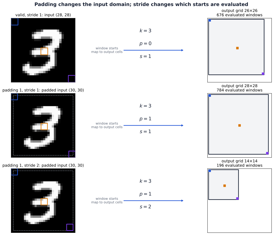
For a \(28\times28\) image and a \(3\times3\) kernel, the tutorial checks three cases:

Padding per side	Stride	Starts along one padded axis	Output spatial shape
\(p=0\)	1	\(0,1,\ldots,25\)	\((26,26)\)
\(p=1\)	1	\(0,1,\ldots,27\)	\((28,28)\)
\(p=1\)	2	\(0,2,\ldots,26\)	\((14,14)\)

In the last two cases, the padded axis has length 30. A padded start of zero corresponds to original-input coordinate \(-1\). Thus padding changes both the available windows and their relationship to the measured image. Stride changes which of those windows are evaluated.

Figure 7: Window starts determine the output grid. The same digit and kernel yield valid, padded, and stride-2 responses with different spatial sizes. Checked tutorial calculations; the MNIST image is attributed to LeCun, Cortes, and Burges under CC BY-SA 3.0.

Shared weights give translation equivariance

Let \(T_{\Delta}\) shift an input by integer displacement \(\Delta=(\Delta_H,\Delta_W)\). \(\Delta_H,\Delta_W\) are the row and column displacements; \(T_\Delta\) names the shift operation. In an idealized image defined on the full integer grid,

\[ (T_{\Delta}\mathbf h)_{a,c} =h_{a-\Delta_H,c-\Delta_W}. \]

To expose the spatial argument, consider one channel and a stride-1 filtering operation \(\mathcal C\) with shared weights and bias. Then

\[ \begin{aligned} \bigl[\mathcal C(T_{\Delta}\mathbf h)\bigr]_{a,c} &=b+\sum_{u,v}W_{u,v} h_{a+u-\Delta_H,c+v-\Delta_W}\\ &=(\mathcal C\mathbf h)_{a-\Delta_H,c-\Delta_W}. \end{aligned} \]

The sums cover the kernel’s offsets. The shifted input presents the same local values to the same coefficients at a correspondingly shifted position. Therefore

\[ \mathcal C(T_{\Delta}\mathbf h) =T_{\Delta}(\mathcal C\mathbf h). \]

This is translation equivariance: transforming the input transforms the output in a predictable way. A pointwise activation also commutes with translation, so adding ReLU does not by itself destroy this stride-1 property. The argument extends to multiple channels because each channel’s local contribution follows the same coordinate shift.

Real images occupy finite grids. Exact correspondence requires matching windows and a compatible boundary convention; cropping, newly introduced padding, or a pattern leaving the image can break it. Within a region where the compared windows contain the same shifted measurements, the local argument still applies.

Translation invariance asks for a different equation. For a classifier \(g\) whose output has no spatial coordinates, the desired property may be

\[ g(T_{\Delta}\mathbf X)=g(\mathbf X). \]

An equivariant map retains where a pattern occurred by moving its response. An invariant class score removes that distinction. Classification may benefit from such stability, while locating an object or predicting a label at each pixel generally needs an output that follows its position. The task determines which property is useful.

NotePause and predict: moving a response

A shifted image produces an equally shifted response map under a stride-one shared filter, away from boundaries. Is that equivariance or invariance? Would an object locator want the response to stay in its old position?

Reveal the explanation

This is equivariance: the output follows the input shift. Invariance would leave the output unchanged. A locator needs position information to follow the object; unchanged coordinates would describe the old location. A classifier may instead benefit from stable class scores after suitable aggregation.

Stride changes the translation relationship

A stride-2 operation samples starts \(0,2,4,\ldots\). Moving a pattern by two input positions aligns it with the next sampled window, corresponding to one output step away from boundaries. Moving it by one input position changes its alignment with the sampling grid.

The simplest counterexample uses a width-1 kernel equal to one and stride 2. For

\[ \mathbf x=[0,1,0,0,0,0], \]

the sampled output is \([0,0,0]\). Shift the input one position right, obtaining \([0,0,1,0,0,0]\), and the sampled output becomes \([0,1,0]\). Translating a zero output cannot produce that nonzero output. Thus the stride-1 equivariance equation cannot be assumed for every one-position shift after subsampling.

Stride reduces the number of evaluated windows and the output resolution. It can make fine positional changes consequential even when the filter itself is shared. In a stack of strided layers, the corresponding aligned input shifts are governed by the product of the strides.

Pooling summarizes a region and loses arrangement

Convolution forms a learned weighted sum. A pooling operation instead applies a fixed summary to each window, normally within each channel independently. For an unpadded \(2\times2\) window \(\mathbf P\), max and average pooling give

\[ \operatorname{MaxPool}(\mathbf P)=\max_{u,v}P_{u,v}, \qquad \operatorname{AvgPool}(\mathbf P)=\frac{1}{4}\sum_{u,v}P_{u,v}. \]

Neither operation adds trainable parameters. A \(2\times2\), stride-2 pool changes a \(28\times28\) map into a \(14\times14\) map, retaining its channel count. The valid-window shape argument applies to this configuration with floor-based output sizes. Other pooling settings require their own conventions; for example, PyTorch’s max-pooling padding uses negative infinity rather than convolution’s default zeros. See PyTorch MaxPool2d.

Max pooling compares signed values, not absolute magnitudes: if every entry is negative, it selects the least negative.

Figure 8: One window contributes one maximum to the pooled map. The highlighted response and destination make the selected value and its position explicit. Checked tutorial calculation on the attributed MNIST image.

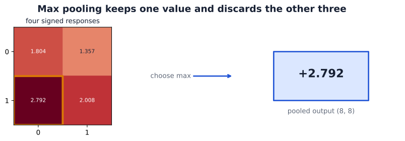
Both the maximum and the mean are unchanged by rearranging values inside the same window. They discard that internal arrangement, but moving values across window boundaries can change the output. For example, width-2, stride-2 max pooling maps \([0,3,2,0]\) to \([3,2]\). A one-position right shift gives \([0,0,3,2]\) and output \([0,3]\). Local pooling therefore does not guarantee translation-invariant predictions.

Pooling also has a backward computation. For a unique maximum, the incoming sensitivity passes to the winning entry while the other entries receive zero from that pooled output. An unpadded four-entry average distributes the sensitivity equally, one quarter to each entry. Tied maxima create a nondifferentiable case that requires an implementation convention. These are still the local-derivative and branch-addition rules from Week 04.

Depth expands structural receptive fields

The biological receptive field was defined by a measured response. In a CNN, we can also ask about possible dependence before observing any response. A structural receptive field describes which input region can affect one output through the architecture’s connections. One width-3 layer uses three input positions. A second local layer combines several such outputs, so its input dependence can extend farther even though neither layer connects globally.

For the tutorial’s two-layer one-dimensional example, the first layer has width 3 and stride 1. Its first two outputs depend on positions \(\{0,1,2\}\) and \(\{1,2,3\}\). A width-2, stride-2 second layer combines these two outputs. Its first output can therefore depend on the union \(\{0,1,2,3\}\): four distinct positions, not six. Its next output combines first-layer positions 2 and 3, depending on \(\{2,3,4,5\}\).

Figure 9: Receptive fields compose through the intermediate layer. Adjacent final outputs have overlapping four-position input regions, with starts separated by two input positions. Course-generated dependency graph from the tutorial.

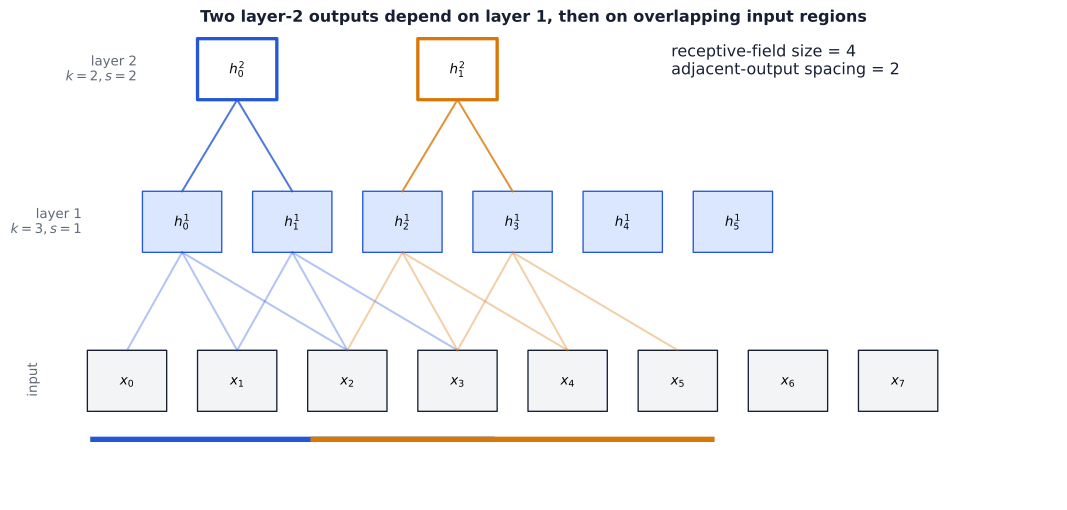
Track two quantities along one spatial axis: \(r_\ell\), the receptive-field extent in input coordinates, and \(j_\ell\), the input-coordinate spacing between adjacent layer-\(\ell\) outputs. Initially one input position sees itself, so \(r_0=j_0=1\).

A width-\(k_\ell\) window spans \(k_\ell\) previous-layer positions. Their first and last starts are separated by \((k_\ell-1)j_{\ell-1}\), and the last position already has extent \(r_{\ell-1}\). Stride \(s_\ell\) multiplies the spacing between evaluated starts. Thus, for a sequential local path with dilation one,

\[ \begin{aligned} r_\ell&=r_{\ell-1}+(k_\ell-1)j_{\ell-1},\\ j_\ell&=s_\ell j_{\ell-1}. \end{aligned} \]

Stage	Kernel width	Stride	Extent \(r\)	Spacing \(j\)
Input	—	—	1	1
First layer	3	1	3	1
Second layer	2	2	4	2

In this example, the dependency sets fill the four-position span. More generally a span can contain unused positions; \(r\) records extent, not necessarily a count of distinct connected measurements. Padding can place part of the nominal span outside the measured image and changes its alignment without changing this extent recurrence. The receptive-field derivation by Araujo, Norris, and Sim treats locations and more general computation graphs in detail; its backward-indexed recurrence describes the same geometry with a different indexing convention.

Important

Structural reach is not measured influence. Zero weights, inactive ReLUs, or max-pooling selections can make some connected inputs have zero local derivative on a particular example. Global aggregation and operations that mix spatial positions or examples require a broader dependency analysis. In particular, training-mode BatchNorm can couple positions through its statistics; the local recurrence alone does not describe that dependence.

For images, apply the recurrence to height and width separately. This supplies the missing geometric explanation for a CNN: depth combines local evidence across larger regions, while stride controls how densely those regions are sampled.

From local features to class logits

A local detector is not yet a classifier. We need to combine local evidence, summarize it across the image, and turn that summary into class scores. Each step has a different job: convolutions construct maps, activations make their composition nonlinear, pooling reduces spatial detail, and the head connects the representation to the task.

A complete architecture has a shape and parameter ledger

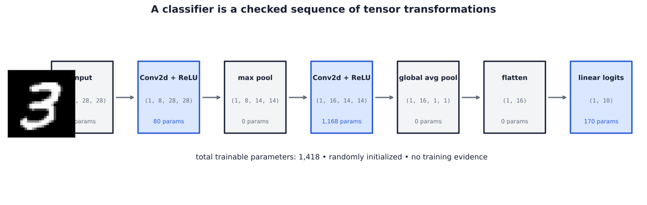
The tutorial’s small classifier receives grayscale \(28\times28\) images. Its first convolution constructs eight activation maps; max pooling halves their spatial size; a second convolution constructs sixteen activation maps. Global averaging then produces one scalar per channel, and a learned linear head produces \(K=10\) logits.

Stage	Output shape	Trainable parameters
Input	\((B,1,28,28)\)	0
\(3\times3\) convolution, padding 1	\((B,8,28,28)\)	80
ReLU	\((B,8,28,28)\)	0
\(2\times2\) max pool, stride 2	\((B,8,14,14)\)	0
\(3\times3\) convolution, padding 1	\((B,16,14,14)\)	1168
ReLU	\((B,16,14,14)\)	0
Global average pool	\((B,16,1,1)\)	0
Flatten per example	\((B,16)\)	0
Linear head	\((B,10)\)	170

The second convolution shows why input channels matter. It owns sixteen filters, each combining eight input channels, giving

\[ 16(8\cdot3\cdot3+1)=1168. \]

The complete model has 1,418 trainable parameters. Pooling and activations alter the computation without adding learned coefficients.

Figure 10: The classifier transforms local activation maps into a vector and then class logits. Shapes and parameter counts describe an untrained architecture, not the usefulness of its representations. Course-generated structural trace from the Week 05 tutorial.

Full-size figure.

The following composition implements the same operations as the tutorial model:

import torch
from torch import nn

torch.manual_seed(202606)
model = nn.Sequential(
    nn.Conv2d(1, 8, kernel_size=3, padding=1),
    nn.ReLU(),
    nn.MaxPool2d(kernel_size=2, stride=2),
    nn.Conv2d(8, 16, kernel_size=3, padding=1),
    nn.ReLU(),
    nn.AdaptiveAvgPool2d((1, 1)),
    nn.Flatten(start_dim=1),
    nn.Linear(16, 10),
)
logits = model(torch.zeros(2, 1, 28, 28))
assert logits.shape == (2, 10)
assert sum(p.numel() for p in model.parameters()) == 1418

The zero input makes this a shape check. The weights remain untrained. Flatten(start_dim=1) keeps the batch axis separate; flattening all axes would incorrectly merge different examples into one vector.

Global averaging connects spatial maps to logits

Let the final activation tensor have shape \((B,C,H',W')\), where \(H',W'\) are its spatial dimensions. Global average pooling constructs a vector \(\mathbf g_n\in\mathbb R^C\) for each example:

\[ g_{n,o}=\frac{1}{H'W'} \sum_{a=0}^{H'-1}\sum_{c=0}^{W'-1}h_{n,o,a,c}. \]

Every channel is averaged separately. The operation preserves a summary of response strength while discarding where within that channel’s map the responses occurred. AdaptiveAvgPool2d((1,1)) gives exactly this one-spatial-cell summary per channel; the API describes the adaptive output shape.

The learned head then computes, for one example represented as a column vector,

\[ \mathbf z_n^{\mathrm{head}} =\mathbf W^{\mathrm{head}}\mathbf g_n+\mathbf b^{\mathrm{head}}, \qquad \mathbf W^{\mathrm{head}}\in\mathbb R^{K\times C}. \]

The head gives each class a learned combination of channel summaries. Channels are not class labels: the example has sixteen summary features and ten output logits. For a batch, the head returns \((B,K)\), consistent with Week 04’s row-major convention. Those logits can be passed directly to the multiclass cross-entropy objective developed there; a hidden-layer ReLU or an extra Softmax is not required after this linear head for that loss.

Permuting spatial entries within a map leaves its mean unchanged. If an input transformation merely permutes each final map’s values, the pooled vector and the head’s logits will therefore be unchanged. An input translation need not have that effect in the complete network: boundaries and strided sampling can alter the values, not just their locations. Global averaging’s invariance to map rearrangement is consequently a conditional route to stable predictions, not a guarantee for every shifted input.

The mean is also unable to recover the discarded arrangement. Two maps with the same channel means can place their strongest responses in different regions yet produce identical head logits. That can be useful for classification, but a task requiring precise locations needs to retain spatial information elsewhere in its architecture.

Trace the local reach before the global operation

Apply the receptive-field recurrence to one axis of the small CNN, omitting pointwise ReLUs because they do not enlarge structural reach:

Stage	Kernel width	Stride	Extent \(r\)	Spacing \(j\)
Input	—	—	1	1
First convolution	3	1	3	1
Max pooling	2	2	4	2
Second convolution	3	1	8	2

One final convolutional position has nominal local reach \(8\times8\), with adjacent positions spaced two original pixels apart. Near borders, some of that reach involves padding. The sixteen channels at a position combine different learned relationships over the same spatial extent.

The classifier is not restricted to one such patch. Global averaging uses all \(14\times14\) positions in each final channel, aggregating their local evidence across the image. In this architecture the union of those local dependencies covers the whole measured input. This statement concerns possible connections: for a particular example, ReLU gates and max-pool winners may leave some pixels without a nonzero local gradient.

Learned hierarchies require evidence beyond a forward pass

Depth permits later filters to combine earlier representations, rather than repeatedly examining raw intensities. An early channel may respond to a local contrast; a later filter can combine several channels and nearby positions. This explains the architectural possibility of a feature hierarchy. It does not assign an interpretable name to every learned channel or show that an untrained model has discovered useful features.

The following example uses an ImageNet-pretrained MobileNetV3-Small on a digit 3 repeated into three channels, resized, and normalized for that model. Six channels per depth were selected by mean absolute activation. It is a separate pretrained model, not the small classifier above.

Figure 11: Stored activations of an ImageNet-pretrained MobileNetV3-Small at four depths for one processed MNIST digit 3. Six channels per depth were selected by mean absolute activation. Reused from the Week 01 tutorial; the MNIST input retains its attribution and CC BY-SA 3.0 terms.

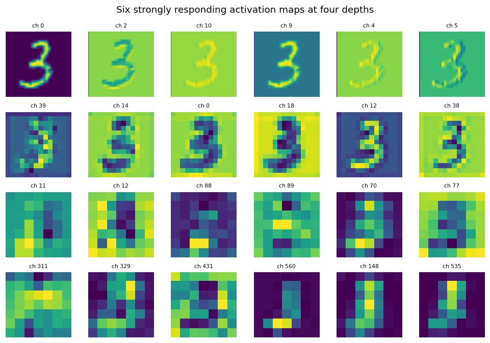
Early maps retain fine spatial structure, while later maps have lower resolution and different response patterns. A high activation does not by itself identify a detector of a particular object part. The chosen channels are a selected view, and brightness across separately displayed maps is not a calibrated comparison of response magnitude. The handwritten digit also differs from the natural-image pretraining domain.

A shape check establishes that a computation fits together. An activation plot shows a particular model’s response. Held-out evaluation tests predictive behavior. These answer different questions about a representation.

The same construction extends to other spatial dimensions

The number in Conv1d, Conv2d, or Conv3d counts axes along which a local kernel slides, not the total rank of the input tensor. Channels remain distinct measurements or learned features at each position.

Operation	Batch layout	Local spatial axes	Example
Conv1d	\((B,C,T)\)	One	Multichannel sampled signal
Conv2d	\((B,C,H,W)\)	Two	RGB image
Conv3d	\((B,C,D,H,W)\)	Three	Volume or video grid

Here \(D\) denotes the third spatial extent, such as volume depth or video time; it is local to this table. A multichannel time series can use Conv1d because its channel axis is combined within each filter rather than scanned as another spatial axis. For Conv3d, a filter instead slides across three spatial coordinates and combines all its input channels at each local neighborhood.

The same architectural hypothesis carries over: nearby values interact, and a useful local rule can be reused at different positions. The later MNIST-1D investigation tests this idea on a one-dimensional synthetic task. Before that, we turn to a different question: how can larger convolutional compositions remain trainable as their depth grows?

Making deeper models trainable

AlexNet: a coordinated design, not just more layers

Our small CNN demonstrates how local features reach a classifier. Scaling that construction requires decisions about optimization, regularization, and computation as well as depth. AlexNet combined five convolutional layers and three fully connected layers with ReLU activations, GPU training, augmentation, weight decay, and dropout. Its 2012 ImageNet result established the practical value of training a large convolutional model on a large labeled dataset (Krizhevsky et al. 2012).

These choices have different jobs. ReLU supplies a nonlinearity whose derivative is one on its positive region, avoiding the progressively small derivatives of saturated sigmoid units there. It can still block gradients on its negative region. Augmentation changes the examples encountered during training; weight decay constrains parameter growth; dropout changes the training computation by randomly suppressing activations. Their effects must be evaluated together with the data and training procedure. A successful historical configuration is evidence about that experiment, rather than a prescription that every visual task needs the same components.

Figure 12: Compact overview of the untrained Torchvision AlexNet variant, traced on a single RGB image of size 224 by 224. Shapes describe a computation, not measured predictive performance.

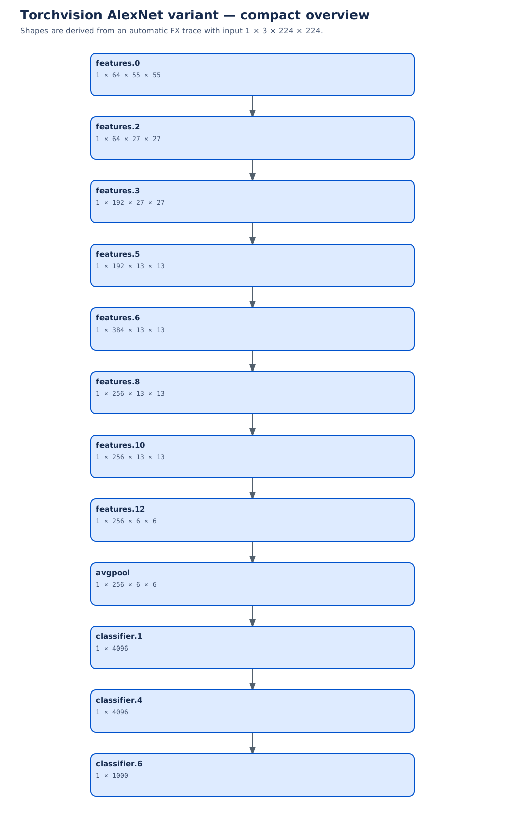
Open the complete AlexNet graph to inspect individual operations and parameter counts. This is the tutorial’s library variant, not an exact reconstruction of the original two-GPU model:

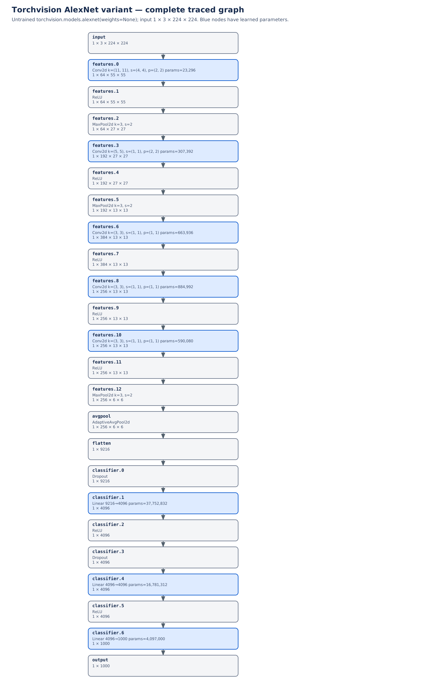
Detail	Original paper	Traced Torchvision variant
Five convolutional widths	96, 256, 384, 384, 256	64, 192, 384, 256, 256
Local response normalization	Included	Absent
Historical GPU split	Restricted some channel connections	No corresponding split

The paper supplies the historical model; the Torchvision source supplies the implementation shown. Local response normalization is a different operation from BatchNorm, introduced below; similar names do not imply interchangeable computations.

The degradation question

Greater representational capacity does not ensure that the optimizer finds a better solution. The ResNet paper demonstrated degradation: some deeper plain networks had higher training error than shallower counterparts (He et al. 2016). Higher training error makes this distinct from a simple overfitting account, in which training fit improves while held-out behavior worsens.

Why is that surprising? Suppose extra blocks have compatible shapes and can represent the identity on the representations they receive. Copy the shallower model’s learned transformations and let each added block pass its input through unchanged. The resulting deeper network computes the same function. Under these assumptions a comparably good solution exists; finding it is a separate optimization problem. The identity construction is conditional: a block that changes dimensions or irreversibly discards information cannot simply copy every input coordinate.

A plain sequence asks the added transformations to learn this pass-through behavior using their ordinary parameters. Residual learning instead makes a direct path explicit. The mathematical question becomes: how much should this block change its input?

Learn a correction to the input

For a block whose input and output shapes match, define

\[ \mathbf y=\mathbf x+F(\mathbf x;\theta_F). \]

Here \(\mathbf x\) is the block input and \(\mathbf y\) its sum, not a dataset target. \(F\) is the learned residual branch and \(\theta_F\) collects that branch’s parameters, a subset of the model’s \(\theta\). If a desired mapping is \(G(\mathbf x)\), the branch would ideally supply \(G(\mathbf x)-\mathbf x\). Setting the branch output to zero makes the sum equal the input.

Figure 13: Identity shortcut in the untrained Torchvision ResNet-18 first residual stage. The input reaches addition through both an unchanged path and a learned two-convolution branch.

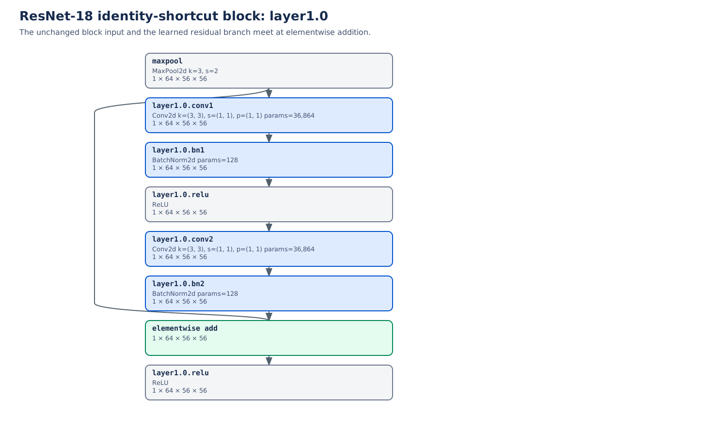
The graph applies ReLU after addition, so the complete block output is \(\mathbf h=\phi(\mathbf y)\). A zero branch then gives \(\phi(\mathbf x)\), which equals \(\mathbf x\) on nonnegative inputs but clips negative coordinates. Keeping the sum separate from its following activation prevents an inaccurate claim of unconditional identity.

The shortcut and branch are added elementwise. They do not concatenate channels. For example, two tensors of shape \((B,64,56,56)\) produce one tensor of that same shape. The identity path contributes no learned parameters, although the addition still performs arithmetic.

Derive the gradient through both paths

Flatten the matching tensor coordinates into column vectors for the derivative calculation. Let \(\mathbf J_F\) have entries \((\mathbf J_F)_{ij}=\partial F_i/\partial x_j\). The identity matrix \(\mathbf I\) has ones on its diagonal and zeros elsewhere. At the sum,

\[ \frac{\partial\mathbf y}{\partial\mathbf x} =\mathbf I+\mathbf J_F. \]

The symbol \(\nabla_{\mathbf y}\) collects derivatives with respect to all coordinates of \(\mathbf y\) into a column gradient. If \(\mathbf g_y=\nabla_{\mathbf y}\mathcal L_{\mathcal B}\) is the downstream gradient, the chain rule gives

\[ \nabla_{\mathbf x}\mathcal L_{\mathcal B} =(\mathbf I+\mathbf J_F)^\top\mathbf g_y =\mathbf g_y+\mathbf J_F^\top\mathbf g_y. \]

This is Week 04’s branch rule: multiply along each path, then add the contributions. The direct path contributes \(\mathbf g_y\) without passing through the branch’s internal derivatives. The branch still receives gradients and learns; the shortcut does not bypass the loss or optimizer.

For a following ReLU, define \(\mathbf D_\phi\) as the diagonal matrix of its coordinate derivatives, away from zero. With \(\mathbf g_h=\nabla_{\mathbf h}\mathcal L_{\mathcal B}\),

\[ \nabla_{\mathbf x}\mathcal L_{\mathcal B} =(\mathbf I+\mathbf J_F)^\top\mathbf D_\phi\mathbf g_h. \]

The activation gate acts before this gradient splits between the paths. At the sum, the identity term can also be cancelled or amplified by the branch. For a scalar branch \(F(x)=ax\), the derivative is \(1+a\): it is one for \(a=0\), zero for \(a=-1\), and three for \(a=2\). A residual route can help optimization without guaranteeing convergence or preventing every vanishing or exploding gradient.

Match shapes when a stage changes

A stage transition often reduces resolution while increasing channels. An identity shortcut cannot add a \((B,64,56,56)\) input to a \((B,128,28,28)\) branch output. Introduce a shortcut mapping \(S\):

\[ \mathbf y=S(\mathbf x)+F(\mathbf x;\theta_F), \qquad \operatorname{shape}(S(\mathbf x)) =\operatorname{shape}(F(\mathbf x)). \]

The paper’s simplified linear projection notation is \(S(\mathbf x)=\mathbf W_s\mathbf x\). In the traced Torchvision stage transition, the shortcut is a stride-two \(1\times1\) convolution followed by BatchNorm. It learns channel combinations and samples a coarser spatial grid. Its parameters and normalization state belong to the model too.

Figure 14: Projection shortcut at the second stage of the untrained Torchvision ResNet-18. Both paths produce 128 channels on a 28-by-28 grid before addition.

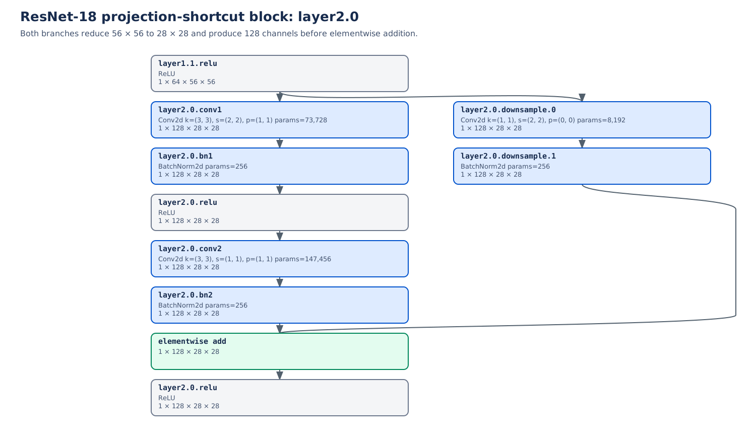
Write \(\mathbf J_S\) for the Jacobian of the shortcut mapping \(S\), defined by the same coordinate-derivative convention as \(\mathbf J_F\). For a projection block the Jacobian at the sum is \(\mathbf J_S+\mathbf J_F\), rather than \(\mathbf I+\mathbf J_F\). If dimensions change, this Jacobian is rectangular. Calling every shortcut an identity would obscure the actual calculation.

Open the identity detail and projection detail at full size to follow each operation. These automatically traced, untrained graphs establish shapes and connections; they provide no evidence of classification accuracy.

Repeat blocks within stages

Figure 15: Compact overview of untrained Torchvision ResNet-18. Four residual stages lead to global average pooling and a learned classifier.

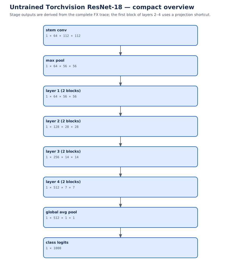
The complete ResNet-18 graph exposes all eight residual additions. Within a stage, blocks repeat at the same spatial resolution. Stage transitions reduce resolution and increase channel count, using projection shortcuts when needed. Deeper family members repeat more blocks or use bottleneck branches, whose \(1\times1\) convolutions change internal channel width around a \(3\times3\) convolution (He et al. 2016).

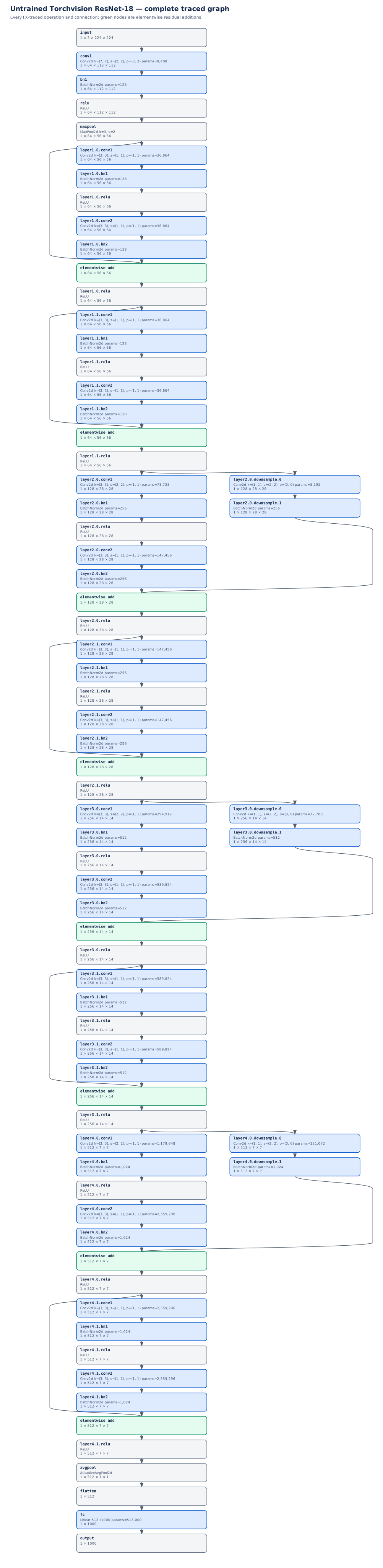
Residual paths address how transformations compose. The BatchNorm nodes in the graphs raise another question: which activation values should determine the scale used by a layer?

Normalization specifies axes and state

A deeper network repeatedly transforms its own intermediate inputs. If activation scales change, the same parameter update can have a different effect downstream. Normalization offers a controlled way to recenter and rescale these intermediate values while allowing the model to learn a useful output scale and offset. It changes the training computation; its benefit still needs validation.

The key question is which values share the statistics. BatchNorm groups a channel’s values across images and spatial positions during training. LayerNorm forms groups within an example. We will first describe their shared operation, then follow the consequences of those different groups.

Center, scale, then learn scale and offset

Let \(\mathcal S\) denote a specified group of \(m\) scalar activation values \(x_j\). \(j\) indexes a member of that group. Define its mean \(\mu_{\mathcal S}\) and population variance \(\sigma^2_{\mathcal S}\) as

\[ \mu_{\mathcal S}=\frac1m\sum_{j\in\mathcal S}x_j, \qquad \sigma^2_{\mathcal S}=\frac1m\sum_{j\in\mathcal S}(x_j-\mu_{\mathcal S})^2. \]

Write \(\widehat{x}_j\) for the normalized value, \(y_j\) for the output, and \(\gamma_j,\beta_j\) for learned scale and offset. The normalize-and-affine construction is

\[ \widehat{x}_j=\frac{x_j-\mu_{\mathcal S}} {\sqrt{\sigma^2_{\mathcal S}+\epsilon}}, \qquad y_j=\gamma_j\widehat{x}_j+\beta_j, \qquad \epsilon>0. \]

The subscripts on \(\gamma_j,\beta_j\) are schematic: a method may share them across many coordinates. They are learned parameters within \(\theta\), whereas the statistics above are computed from activations. The positive constant \(\epsilon\) keeps the denominator nonzero and limits scaling when variance is small. Batch normalization introduced this construction with batch-based groups and learned affine flexibility (Ioffe and Szegedy 2015).

Two properties follow directly. Centered values sum to zero over their group. Their normalized population variance is

\[ \frac{\sigma^2_{\mathcal S}}{\sigma^2_{\mathcal S}+\epsilon}, \]

which is less than one for finite positive variance and positive \(\epsilon\). A constant group has zero normalized values. The learned affine step can change both mean and variance again; it does not enforce standardized final outputs.

Normalization also changes the derivative structure. Since \(\partial\mu_{\mathcal S}/\partial x_k=1/m\), changing one member changes the centering of other members, and generally changes their scaling through the variance. Thus a coordinate’s output can depend on the entire statistics group. The group is an architectural choice, not an incidental implementation detail.

BatchNorm on an image tensor

For \(\mathbf X\in\mathbb R^{B\times C\times H\times W}\), training-mode convolutional BatchNorm uses one group per channel. Write \(M=BHW\) for the number of values in each statistics group, and \(Y\) for the normalized-and-affine output tensor. Then

\[ \begin{aligned} \mu_c&=\frac1M\sum_{n,a,v}X_{n,c,a,v},\\ \sigma_c^2&=\frac1M\sum_{n,a,v}(X_{n,c,a,v}-\mu_c)^2,\\ Y_{n,c,a,v}&=\gamma_c\frac{X_{n,c,a,v}-\mu_c} {\sqrt{\sigma_c^2+\epsilon}}+\beta_c. \end{aligned} \]

Here \(n,a,v\) index examples, rows, and columns. Channels stay separate: an RGB-like channel with a large mean does not contribute directly to another channel’s mean. Each learned pair \((\gamma_c,\beta_c)\) is reused at every spatial location and for every example. With affine parameters enabled, there are \(2C\) trainable scalars.

A simple channel group containing values \(1,3,5,7\) has mean four and variance five. With \(\gamma=1\), \(\beta=0\), its outputs are \(( -3,-1,1,3)/\sqrt{5+\epsilon}\). If the first example supplies \(1,3\) and the second supplies \(5,7\), changing the second example changes the first example’s normalized values. This is batch coupling, even though the convolution before it may act independently on each image.

It also qualifies our earlier receptive-field calculations. During training, BatchNorm statistics connect all locations and examples in a channel. The local convolution/pooling recurrence still describes those local paths, but does not describe every dependency introduced by normalization. At evaluation with fixed statistics, BatchNorm instead applies a fixed affine transformation to each coordinate.

Running statistics are model state

The default PyTorch BatchNorm2d(C) keeps running mean and variance estimates during training, then uses them in evaluation. These estimates are buffers, not parameters updated by the optimizer. Consequently the default model’s behavior depends on both learned parameters and accumulated state.

The running estimates are updated from training batches. Their update conventions are documented in PyTorch BatchNorm2d. With the nondefault track_running_stats=False, evaluation also uses current-input statistics.

Three controls affect different parts of this process:

Control	What it changes	Independent behavior
model.eval()	Mode-sensitive modules, including BatchNorm and dropout	Gradient recording can remain enabled
torch.no_grad()	Recording operations for automatic differentiation	Training-mode running statistics still update
parameter.requires_grad_(False)	Whether that parameter accumulates gradients	Module mode and buffer updates remain separate

For example, a training-mode BatchNorm forward pass inside no_grad() still updates its buffers. Conversely, an evaluation-mode forward pass can still be differentiated. The official autograd notes distinguish evaluation mode from gradient modes. We will use this distinction when adapting a pretrained backbone below.

Small or highly correlated training groups can yield unrepresentative statistics. Batch size one is not automatically a single-value group: a spatial channel still supplies \(HW\) values, although neighboring positions may be strongly correlated. A group with only one value cannot supply an unbiased sample variance. At deployment, stored statistics may also poorly describe a shifted input distribution. These are reasons to inspect axes, mode, and data together, rather than assuming normalization removes distribution differences.

LayerNorm: a worked single-example calculation

Layer normalization builds its groups within each example rather than across examples (Ba et al. 2016). The lecture’s deliberately small example makes the affine step and \(\epsilon\) visible. For \(\mathbf x=(1,3)\),

\[ \mu=2,\qquad \sigma^2=1,\qquad \widehat{\mathbf x}=\frac{(-1,1)}{\sqrt{1.25}} \approx(-0.894427,0.894427), \]

using \(\epsilon=0.25\). Apply \(\gamma=(2,0.5)\) and \(\beta=(1,-1)\) coordinatewise:

\[ \mathbf y=\left(1-\frac2{\sqrt{1.25}},\; -1+\frac{0.5}{\sqrt{1.25}}\right) \approx(-0.788854,-0.552786). \]

The normalized pair has mean zero and variance \(1/1.25=0.8\). Its final affine output has neither zero mean nor unit variance. The large \(\epsilon\) is a teaching choice, not a proposed training setting.

The following standalone calculation translates those values directly into PyTorch:

import torch
from torch import nn

x = torch.tensor([[1.0, 3.0]], dtype=torch.float64)
normalizer = nn.LayerNorm(2, eps=0.25).double()
with torch.no_grad():
    normalizer.weight.copy_(torch.tensor([2.0, 0.5]))  # gamma
    normalizer.bias.copy_(torch.tensor([1.0, -1.0]))   # beta
output = normalizer(x)
expected = torch.tensor([[-0.788854382, -0.552786405]],
                        dtype=torch.float64)
torch.testing.assert_close(output, expected, atol=1e-8, rtol=0)

No other example enters these statistics. Adding another example to the batch leaves this example’s output unchanged when its values and affine parameters stay fixed.

State the trailing axes explicitly

In PyTorch, normalized_shape specifies the trailing dimensions reduced by LayerNorm and the shape of its affine parameters. Input statistics are used in both train and eval modes; there are no BatchNorm-style running estimates. The variance uses the population convention. See PyTorch LayerNorm.

Input layout and call	Statistics group	Default affine shape	Trainable scalars
\((B,C,H,W)\); LayerNorm((C,H,W))	All channels and pixels of each image	\((C,H,W)\)	\(2CHW\)
\((B,C,H,W)\); LayerNorm((H,W))	Spatial map of each example/channel pair	\((H,W)\)	\(2HW\)
\((B,N,D)\); LayerNorm(D)	Features of each example/token pair	\((D)\)	\(2D\)

In the token row, \(N\) counts sequence positions and \(D\) is the feature-vector width, replacing its earlier Conv3d meaning. We return to tokens in Week 06.

The first two image calls express different hypotheses. Whole-image normalization measures every channel and position together, while spatial-map normalization keeps channels in separate statistics groups. Its spatial affine parameters are shared over leading batch and channel axes. Whole-image LayerNorm also fixes a parameter shape containing the chosen resolution.

On a channel-first \((B,C,H,W)\) tensor, LayerNorm(C) does not select the channel axis. It expects the final dimension to have size \(C\) and reduces that final dimension. If \(W=C\), it can even run successfully while normalizing width rather than channels. To normalize channels at each pixel with this API, channels must be placed last, producing \((B,H,W,C)\), before applying LayerNorm(C).

NotePause and predict: another example joins the batch

Keep one image and the affine parameters fixed, but replace another image in its batch. Can its training-mode BatchNorm output change? What about whole-image LayerNorm? Assume default running-statistic tracking when considering evaluation.

Reveal the explanation

Training-mode BatchNorm can change because each channel’s statistics include other examples. Whole-image LayerNorm uses only that image’s coordinates, so the replacement does not change its output. Default evaluation-mode BatchNorm uses stored statistics, so changing another current input does not change the fixed image’s output either.

Choose a grouping that fits the intended computation

BatchNorm shares per-channel statistics across examples and locations during training; LayerNorm groups selected coordinates within each example. A change that affects every value of a statistics group equally is partly removed by centering and scaling before the affine step. Whether that variation is nuisance or useful signal depends on the task and representation.

Normalization is therefore an architectural hypothesis to compare on validation data. Check the actual batch composition, tensor layout, parameter shape, and inference behavior. A CNN with representative batches may use BatchNorm effectively; token features often use LayerNorm over their embedding width. Neither observation establishes a universal replacement rule, and a model without normalization remains a useful baseline.

Residual connections and normalization alter how a deep representation is learned and evaluated. Once a representation has been learned, reusing it introduces a related practical question: which parameters, buffers, and mode-dependent operations should change on the new task?

Reusing representations responsibly

Augmentation asserts something about the target

A training example is more than an array: it includes a target whose meaning determines which changes are acceptable. For an object-class task, reflecting a photograph of a cat can preserve its class. For a direction-sign task, reflection turns a left-pointing arrow into a right-pointing arrow. Keeping the original direction label would introduce incorrect supervision.

Let \(T\) be an input transformation and let \(y(\mathbf x)\) denote the task’s target function. Training on \((T(\mathbf x),y(\mathbf x))\) asserts

\[ y(T(\mathbf x))=y(\mathbf x). \]

The assertion is task-specific. For localization or segmentation, a geometrically valid transformation generally requires transforming the target too: a reflected image needs reflected coordinates or a reflected mask. An unchanged classification label and a transformed spatial target are different supervision rules.

Augmentation exposes the learner to variation that we want it to handle. It does not prove exact invariance of the resulting model. Its transformations should preserve the relevant target and plausibly represent variation in the intended use. A crop that removes the only labeled object, or a color change that erases diagnostic color evidence, can violate that requirement. AlexNet’s augmentation choices provide a historical example of task-specific regularization (Krizhevsky et al. 2012), not a universal list of safe transformations.

Choose augmentation during development using validation evidence. Check errors under the proposed transformations, including cases whose labels might change. Applying transformations indiscriminately can teach the model to ignore precisely the distinction the task needs.

Freeze a representation, then learn a new head

Suppose we want to classify satellite scenes using a network pretrained on another image collection. We can reuse its image-to-feature computation and fit a new classifier for our labels. The reused part is the backbone; the new task-specific classifier is the head.

Decompose a pretrained model into a backbone \(f_{\theta_{\mathrm{back}}}\) and a task head \(q_{\theta_{\mathrm{head}}}\). The subscripts \(\mathrm{back}\) and \(\mathrm{head}\) distinguish the two parameter collections; \(\mathbf z^{\mathrm{head}}\) denotes the head’s logits. For one input,

\[ \mathbf h=f_{\theta_{\mathrm{back}}}(\mathbf x), \qquad \mathbf z^{\mathrm{head}}=q_{\theta_{\mathrm{head}}}(\mathbf h). \]

In frozen-feature transfer, the backbone supplies a fixed representation and only the new head is optimized on the target task. For a linear head, \(\mathbf z^{\mathrm{head}}=\mathbf W^{\mathrm{head}}\mathbf h+\mathbf b^{\mathrm{head}}\), this asks whether the supplied features support a linear class boundary. A nonlinear head tests a broader form of usability, so its result should not be described as evidence of linear separability.

A fixed representation requires a complete state policy. Freeze backbone parameters, keep its BatchNorm running statistics fixed, and disable training-mode dropout. Use the preprocessing specified for the pretrained weights: channel order, input scaling, resizing, and normalization are part of the input contract. Otherwise the backbone may receive measurements different from those on which its features were learned.

A practical implementation disables gradients for backbone parameters, puts the backbone in evaluation mode, and optimizes only the head. Its forward pass may use no_grad() around the backbone when input gradients are unnecessary, but must leave the head’s computation differentiable. If a wrapper’s train() call switches the backbone back to training mode, reapply its evaluation policy before the next forward pass. See the PyTorch autograd notes.

Features can be cached when both the backbone and preprocessing are fixed. If random augmentation produces different inputs, one cached vector per original example does not represent every augmented view. Changes in preprocessing or backbone state also invalidate the cached representation.

Frozen transfer is a useful starting experiment when target labels or compute are limited. Its success depends on the relation between source features and target distinctions. Yosinski and colleagues found that feature specialization and splitting co-adapted layers can limit transfer, with transferability decreasing as source and target tasks diverged in their experiments (Yosinski et al. 2014). A pretrained feature extractor is a hypothesis to evaluate, not a guarantee that its source task supplied everything the new task needs.

Adapt only as much as validation supports

Fine-tuning allows selected pretrained parameters to change under the target objective. Its gradient again passes through the updated parts of the backbone. Remove the relevant no_grad() boundary when unfreezing those parts, and ensure their parameters belong to the optimizer. A parameter with gradients that the optimizer never sees will not receive the intended update.

Strategy	Parameters updated	Question being tested
Head only	New task head	Are the existing features already usable?
Partial fine-tuning	Head and selected later blocks	Does adapting later representations help?
Full fine-tuning	Head and entire backbone	Does broader adaptation justify its cost and risks?

Head-only training may fail through representation mismatch; broader adaptation can overfit a small target dataset or disrupt useful features. Partial adaptation also creates a boundary between fixed and changing representations. Specify the normalization policy at that boundary instead of allowing a blanket mode change to decide it accidentally.

Starting with the head and then testing later-block adaptation is a practical route, not a mandatory sequence. Smaller learning rates for pretrained parameters are a starting heuristic. Compare strategies on the same target validation split with recorded budgets and preprocessing, including a credible baseline. Reserve the test split for the chosen procedure; do not use it to choose how many blocks to unfreeze.

Predictive evidence extends beyond an average score

Held-out accuracy answers a specified question about a specified sample. It does not establish that the model uses the intended evidence or remains reliable under a new device, background, or population. Inspect class-level failures and errors under realistic changes. For example, changing the background while retaining an object can reveal prediction sensitivity worth investigating; it does not by itself prove that all background information is irrelevant.

Develop probes on validation data, state what they preserve, and distinguish exploratory diagnosis from final evaluation. Probabilities and calibration matter when confidence affects a decision; uncertainty across examples and training seeds matters when comparing models. Our next investigation deliberately addresses a narrower question with a small synthetic benchmark and a documented protocol.

Worked investigation: MLP versus Conv1d

Does a model that reuses local patterns learn a useful representation under the same update budget as a dense alternative? Ordered signals provide a small test of that hypothesis. We compare an MLP and a Conv1d model on the same examples. These are complete model designs, so their comparison will not isolate sharing alone.

A label names a generating waveform

MNIST-1D is a synthetic task by Sam Greydanus and Dmitry Kobak. Its labels 0–9 identify generating templates; the inputs are noisy, transformed length-40 signals, not flattened handwritten digit images. The official construction at the tutorial’s pinned revision uses mechanisms including padding, translation, scaling, shear, and correlated and independent noise. We cannot infer the exact random transformation parameters of a displayed example simply by looking at its waveform.

Figure 16: Ten official clean MNIST-1D templates and three supplied training signals from class 3. Class labels identify synthetic generating shapes. Reused tutorial figure; data attribution to Greydanus and Kobak under Apache-2.0.

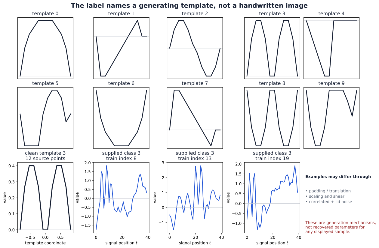
Full-size figure. Nearby signal positions have meaning because they describe an ordered shape. This gives locality and sharing a plausible role, while transformations and noise make direct template recognition nontrivial.

This section reports the tutorial’s stored experiment and figures. The notebook records the data files and reproducibility details.

Separate the roles of training, validation, and test

The notebook uses seed 202605 to construct a stratified 3,200/800 split from the supplied 4,000 training cases. Stratification approximately preserves class proportions, rather than assuming every class has exactly the same count. The supplied 1,000 test cases retain their separate role.

Preprocessing fits one scalar mean and one scalar population standard deviation over all entries of the 3,200 training signals. The same transformation is applied to every split. Fitting these values on validation or test data would let held-out examples influence development. This input preprocessing is separate from normalization of hidden activations.

Split	Cases	Role
Training	3,200	Fit preprocessing and update parameters
Validation	800	Compare development behavior and select checkpoints
Supplied test	1,000	Evaluate both fixed selected checkpoints

Similar parameter counts, different connectivity

Both models receive the same normalized numbers and output ten logits. The MLP receives \((B,40)\) and uses a 40-to-68 linear layer, ReLU, and a 68-to-10 head. Its parameter count is

\[ 68(40+1)+10(68+1)=3478. \]

The Conv1d model views the input as \((B,1,40)\). Its three stride-one, zero-padded convolutional layers have 16 output channels and kernel widths 5, 5, and 3, each followed by ReLU. Length remains 40 throughout. Adaptive average pooling then produces eight ordered cells per channel, which are flattened into 128 head inputs.

Conv1d stage	Output shape	Parameters
Width 5, padding 2, 1-to-16 channels	\((B,16,40)\)	\(16(1\cdot5+1)=96\)
Width 5, padding 2, 16-to-16 channels	\((B,16,40)\)	\(16(16\cdot5+1)=1296\)
Width 3, padding 1, 16-to-16 channels	\((B,16,40)\)	\(16(16\cdot3+1)=784\)
Adaptive average pool	\((B,16,8)\)	0
Flatten and 128-to-10 head	\((B,10)\)	\(10(128+1)=1290\)

The total is \(96+1296+784+1290=3466\). ReLUs add no parameters. The two counts differ by twelve, but comparable counts do not make their function classes, depth, optimization behavior, or compute identical.

Figure 17: Before training, one Conv1d channel has a banded effective operator with repeated coefficients, while the MLP has independently adjustable dense connections. Reused initialized-model figure from the tutorial.

Full-size figure.

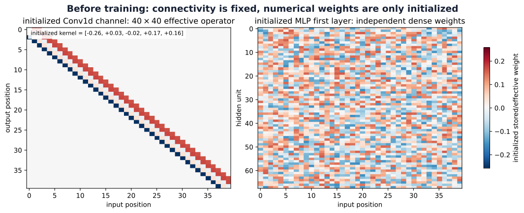
The banded operator’s repeated entries come from only five stored kernel weights, plus one bias. The dense layer instead adjusts each connection independently. This illustrates architectural structure before training.

The receptive-field recurrence gives extents 5, 9, and 11 through the local Conv1d stack, with spacing one. A final position can use an eleven-position span, qualified by padding near boundaries. The classifier combines many such positions: pooling 40 values into eight cells averages consecutive groups of five in this divisible case. Each interior pooled cell can cover a nominal fifteen-position span, from five overlapping eleven-position dependencies. The final linear head uses all cells and can depend on the whole signal.

Unlike global pooling to one cell, this eight-cell pooling retains coarse ordered location. Head weights can treat different cells differently. The model therefore should not be described as exactly translation-invariant; its boundaries and retained spatial bins also matter. See PyTorch AdaptiveAvgPool1d for the output-shape contract.

Match the protocol, then state what remains unmatched

The notebook precomputes one sequence of shuffled training orders and uses it for both models. Each epoch contains \(3200/64=50\) mini-batch updates. Thirty epochs give 1,500 updates per model, using mean cross-entropy and Adam with learning rate \(10^{-3}\). Both initializations use seed 202605; equal seeds make the procedure reproducible but do not supply equivalent initial representations to different architectures.

After each epoch, training and validation metrics are computed in evaluation mode on their respective complete splits. Thus the plotted training loss is an epoch-end evaluation of the current model, not an average of the changing losses observed during updates. For each model the checkpoint with minimum validation loss is retained. Only after both selected states are fixed does the notebook evaluate each once on the supplied test split.

The protocol matches examples, order, optimizer setting, batch size, update count, and selection rule. It does not match arithmetic operations or wall-clock cost. Similar parameter counts also leave depth, aggregation, and connectivity different. The comparison evaluates these two complete model designs under this procedure; it does not isolate the causal contribution of sharing alone.

Figure 18: Stored training and validation curves for the two models across the fixed 30-epoch budget. Both minimum-validation-loss checkpoints occur at epoch 30. This is one split and seed, with no repeated-run uncertainty band.

Full-size figure.

NotePause and predict: the last checkpoint wins

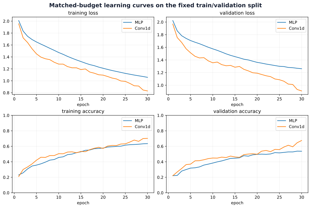
Both MNIST-1D models select epoch 30, the last allowed epoch. Does that show that they have converged? Which evidence in the figure should guide your answer?

Reveal the explanation

No. Both validation-loss curves are still falling at the budget boundary. Selection at the final epoch identifies the best checkpoint seen under this budget; it does not show that further training would cease to help. Investigate a longer development budget on validation data, keeping test results out of that decision.

Read the stored outcomes and paired failures

The notebook reports the following rounded values for its selected checkpoints:

Model	Selected epoch	Validation loss	Validation accuracy	Test loss	Test accuracy
MLP	30	1.2615	0.536	1.2424	0.521
Conv1d	30	0.9097	0.675	0.9023	0.654

Conv1d has higher accuracy and lower loss in this stored comparison. The result is consistent with useful local shared structure on these generated signals. It does not rank all CNNs above all MLPs, measure performance on handwritten digit images, or establish an effect averaged across seeds and splits.

Separate accuracy values can hide which examples each model gets right. The paired test categories preserve that relationship:

Outcome on the same test example	Count
Both correct	416
Only MLP wrong	238
Only Conv1d wrong	105
Both wrong	241

There are 105 cases where MLP is correct and Conv1d is wrong. The stronger aggregate score therefore does not mean better predictions on every input. The two disagreement categories show where the models differ; the shared-error category points to remaining difficulty.

Figure 19: One deterministically selected example from each paired test category, with true labels and both predictions. Reused tutorial output; this is descriptive analysis after the fixed test evaluation, not a checkpoint-selection tool.

Full-size figure.

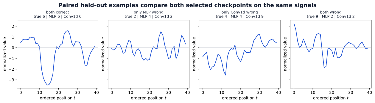
The gallery selects the first available case in each category, not a random or representative sample of the category. It can suggest questions about failures, but four examples cannot establish a systematic class or transformation pattern. Such claims need broader error analysis and a development protocol that keeps further tuning separate from final evaluation.

The defensible conclusion is bounded: on this synthetic benchmark, split, seed, and 30-epoch protocol, the selected Conv1d model outperformed the selected MLP. Repeated seeds, additional splits, credible tuning of both designs, and separate compute comparisons would address questions that this single experiment leaves open.

Synthesis, exercises, and further reading

What the chapter establishes

A convolutional network retains Week 04’s learning machinery while constraining its affine transformations. Locality limits the inputs used at one position; sharing reuses coefficients across positions; channel summation combines different measurements. The chain rule accumulates contributions from every shared use into one compact parameter gradient.

Geometry determines how that computation meets the input. Padding supplies boundary values, stride selects window starts, and pooling summarizes regions. Depth expands local structural reach; global or coarse aggregation connects spatial evidence to a task head. Equivariance means that outputs follow transformations, while invariance means that the task output stays unchanged. Neither pooling nor a familiar architecture name guarantees the latter.

Residual paths provide a direct route alongside learned transformations. Normalization groups activation coordinates and may carry state. Augmentation asserts a target-preserving relationship, and transfer learning decides which learned parameters and accumulated state to preserve or adapt. Each choice changes what the model can represent or how it learns. Validation evidence tests those choices; held-out evaluation supports a specified final claim.

Common confusions to resolve

Confusion	Distinction to keep
A channel is a class	Hidden channels are features; the task head produces class logits
Fewer parameters guarantee faster or better training	Counts describe stored degrees of freedom; compute and predictive evidence need separate checks
Receptive-field extent equals active influence	Extent describes possible local connections; gates, weights, and normalization alter actual dependence
An identity shortcut guarantees an identity block	Addition, the residual branch, and a following activation all affect the output
Frozen parameters mean fixed features	Buffers, dropout mode, and preprocessing also determine the representation
A test-set win establishes a general model ranking	The claim is bounded by the dataset, split, training procedure, and uncertainty examined

Exercises

These optional exercises extend the explanations without supplying solutions. Exercises 1–2 return to convolution and learning; 3–4 to geometry; 5–6 to depth and normalization; 7–8 to transfer and augmentation; and 9 to the experiment.

Exercise 1 — A complete convolution ledger

An input has shape \((B,3,32,32)\). A convolution uses twelve output filters, a \(5\times5\) kernel, stride two, symmetric zero padding two, and a bias. Derive both spatial output dimensions and the parameter count. Explain why changing \(B\) changes neither the spatial shape nor the number of learned coefficients. State the weight-tensor shape and the number of input-channel slices per filter.

Exercise 2 — Shared gradients with unequal sensitivities

For \(\mathbf x=(2,-1,3,0)\) and a width-2 kernel \(\mathbf w=(1,2)\), use stride one, no padding, and no bias. Compute all three outputs. Let \(J=z_0+2z_1-z_2\). Derive both kernel gradients by adding the contributions from each use, and check them with autograd. Explain why summing unweighted input windows would give the wrong answer here.

Exercise 3 — Trace extent and spacing

Along one axis, compose a width-3, stride-2 convolution; a width-2, stride-2 pool; and a width-3, stride-1 convolution. Trace receptive-field extent and output spacing after each operation. Explain which additional information is needed to locate the receptive field of a particular output near a boundary. Distinguish nominal extent from a count of measured inputs.

Exercise 4 — A translation claim needs a domain

Construct a one-dimensional example where stride-2 sampling changes under a one-position shift in a way that cannot be described as an output translation. Then identify an aligned shift that does correspond to an output shift away from boundaries. Explain why global averaging cannot repair every boundary or sampling discrepancy introduced earlier in a classifier.

Exercise 5 — Residual paths and gates

Let \(F(\mathbf x)=\mathbf A\mathbf x\) with \(\mathbf A=\begin{bmatrix}0&1\\-1&0\end{bmatrix}\) and \(\mathbf x=(2,1)^\top\). Compute the residual sum, the post-addition ReLU output, and the input gradient of \(J=h_0+3h_1\). Use the column-gradient convention. Compare with the gradient when ReLU is omitted and explain the difference through the two paths and their gate.

Exercise 6 — Axes and parameters

For a tensor \((B,C,H,W)=(4,8,6,6)\), specify the statistics groups and affine-parameter counts for BatchNorm2d(8), LayerNorm((8,6,6)), and LayerNorm((6,6)). Which outputs may change if a different example joins the training batch? Which methods keep running statistics? Explain why LayerNorm(8) does not select channels on this layout.

Exercise 7 — Audit a frozen backbone

A wrapper contains a frozen backbone with BatchNorm and dropout, and a trainable head. Its training loop calls wrapper.train() before every epoch. Explain why requires_grad=False on backbone parameters does not establish fixed features. Propose a mode and optimizer policy, then verify with before/after copies that one update changes the head while preserving every backbone parameter and buffer.

Exercise 8 — Decide whether an augmentation is valid

Consider horizontal reflection for object classification, direction-sign classification, and segmentation. For each, state whether the target should remain fixed, change, or require case-specific inspection. Describe a validation probe that could detect an inappropriate invariance assumption without using the test set for development.

Exercise 9 — What would the next experiment answer?

Using the stored MNIST-1D curves and paired counts, state one supported result and three questions the run does not answer. Design a follow-up on validation data that investigates one question: longer training, seed variability, an ablation of sharing, or equal-compute comparison. Specify the factors held fixed, selection rule, and final evaluation boundary. Explain why similar parameter counts alone do not isolate locality or sharing.

Further reading

Read primary sources with a particular question in mind:

• AlexNet: how do architecture, optimization, augmentation, and hardware work together, and which details differ from the library variant? (Krizhevsky et al. 2012)
• ResNet: what training-error evidence motivates residual learning, and when do shortcut dimensions need adjustment? (He et al. 2016)
• BatchNorm and LayerNorm: which values supply the statistics, which parameters are learned, and how do training and evaluation differ? (Ioffe and Szegedy 2015; Ba et al. 2016)
• Feature transfer: how do source-task specialization and the boundary between transferred and adapted layers affect reuse? (Yosinski et al. 2014)
• The official MNIST-1D repository at the pinned revision: how does the generation pipeline make spatial biases experimentally relevant?
• Vision Transformer: how can an image become a sequence of embedded patches, and what role does position information play? (Dosovitskiy et al. 2021)

Looking ahead: sequences and attention

Convolution has already shown one way to process an ordered signal with shared parameters. The next week develops sequential representations, recurrent states, and attention. These methods retain the same objective, chain rule, and validation responsibilities while changing how positions interact.

Vision Transformers provide one bridge: image patches become tokens, position information is represented explicitly, and self-attention can connect distant patches. The original ViT study examined this construction at substantial pretraining scales (Dosovitskiy et al. 2021); it does not establish a timeless architecture ranking. Local filters, recurrence, and attention make different assumptions about interactions. Understanding those assumptions will let us compare their behavior rather than choose solely from their names.

Ba, Jimmy Lei, Jamie Ryan Kiros, and Geoffrey E. Hinton. 2016. “Layer Normalization.” arXiv Preprint arXiv:1607.06450. https://arxiv.org/abs/1607.06450.

Dosovitskiy, Alexey, Lucas Beyer, Alexander Kolesnikov, et al. 2021. “An Image Is Worth 16x16 Words: Transformers for Image Recognition at Scale.” International Conference on Learning Representations. https://arxiv.org/abs/2010.11929.

He, Kaiming, Xiangyu Zhang, Shaoqing Ren, and Jian Sun. 2016. “Deep Residual Learning for Image Recognition.” Proceedings of the IEEE Conference on Computer Vision and Pattern Recognition, 770–78. https://openaccess.thecvf.com/content_cvpr_2016/html/He_Deep_Residual_Learning_CVPR_2016_paper.html.

Hubel, David H., and Torsten N. Wiesel. 1959. “Receptive Fields of Single Neurones in the Cat’s Striate Cortex.” The Journal of Physiology 148 (3): 574–91. https://doi.org/10.1113/jphysiol.1959.sp006308.

Ioffe, Sergey, and Christian Szegedy. 2015. “Batch Normalization: Accelerating Deep Network Training by Reducing Internal Covariate Shift.” Proceedings of the 32nd International Conference on Machine Learning 37: 448–56. https://proceedings.mlr.press/v37/ioffe15.html.

Krizhevsky, Alex, Ilya Sutskever, and Geoffrey E. Hinton. 2012. “ImageNet Classification with Deep Convolutional Neural Networks.” Advances in Neural Information Processing Systems 25. https://papers.nips.cc/paper_files/paper/2012/hash/c399862d3b9d6b76c8436e924a68c45b-Abstract.html.

Yosinski, Jason, Jeff Clune, Yoshua Bengio, and Hod Lipson. 2014. “How Transferable Are Features in Deep Neural Networks?” Advances in Neural Information Processing Systems 27. https://papers.nips.cc/paper_files/paper/2014/hash/532a2f85b6977104bc93f8580abbb330-Abstract.html.