Frequentist and
Bayesian approaches
to ML

Week-07 · ML-2026

From likelihood and losses
to latent-variable inference

Alexei Kornaev,
Dr. Sc., Prof.

Innopolis University

Researcher at the RC for AI,
National RC for Oncology n.a. N.N. Blokhin

The elephant illustration previews learning from incomplete evidence. Its curves are conceptual, not calibrated posterior computations. Do not imply that every observation necessarily reduces uncertainty. The probability section will make the assumptions and update rule explicit.

What will we understand and then test?

Recap: finish the scalar RNN backward pass.

1. Probability: describe what is uncertain
2. Likelihood: explain the loss
3. Bayesian inference: update with evidence
4. KL: compare distributions
5. VAE: infer a hidden cause and generate

Explain familiar losses, compare inference approaches, and read a VAE. Tutorial: test the argument with rainfall and images.

Notation for today’s route

Symbols	Meaning
$\theta$; $z_t,h_t,\phi$; $g_v=\partial L/\partial v$	Model weights; RNN preactivation, state, activation; loss derivative
$P(A)$; $p$; $\mathbb E$	Event probability; stated mass/density model; expectation
$\mathcal D=\{(x_i,y_i)\}_{i=1}^n$; $L_i,L$	Observed data; per-observation loss and summed loss
$\sigma^2$; $\tau^2$	Observation-noise variance; weight-prior variance
$u,\psi,q_\psi(u\mid x)$; $\mathcal E$	VAE latent coordinates, encoder weights, approximate posterior; ELBO

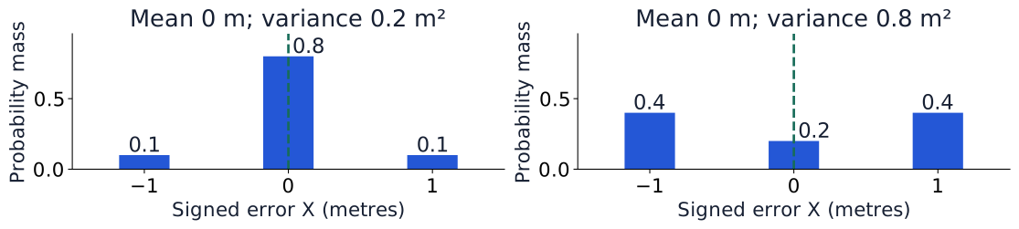
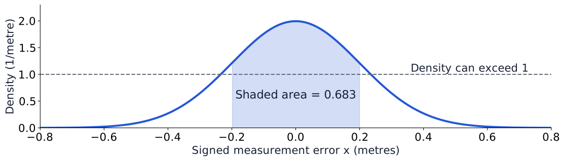
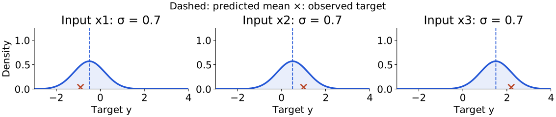
Identify the variable, what is observed, and which distribution supplies the average.

Natural logs and nats; reductions are stated explicitly. Specialized symbols and tensor shapes are defined beside first use. VAE paper $z,\phi$ translate to $u,\psi$ here.

Before probability: one scalar RNN

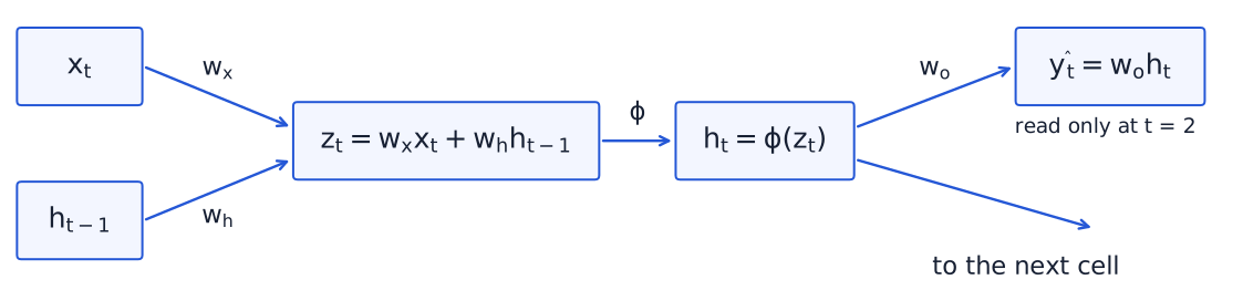
One input coordinate. One state coordinate. Three shared weights.

Trace a prediction forward, then follow its loss backward.

Week 06 textbook: the scalar recurrent model. Same model and notation; new illustrative numbers below.

Separate the cell from the prediction

$$z_t=w_xx_t+w_hh_{t-1},\qquad h_t=\phi(z_t),\qquad x_t,h_t\in\mathbb R.$$

Repeated cell: shared $w_x,w_h$.
Initial state: fixed $h_{-1}=0$.

Final readout: $\widehat y=w_oh_2$.
Trainable weights: $\theta=(w_x,w_h,w_o)$.

The state travels through time; the readout makes the prediction.

Both biases are fixed at zero. This example has one target and one final loss.

Forward: three cells, one final loss

Fixed $h_{-1}=0$; shared $w_x,w_h$; any differentiable activation $\phi$.

Cell 0

$$z_0=w_xx_0+w_hh_{-1}$$ $$h_0=\phi(z_0)$$

Cell 1

$$z_1=w_xx_1+w_hh_0$$ $$h_1=\phi(z_1)$$

Cell 2

$$z_2=w_xx_2+w_hh_1$$ $$h_2=\phi(z_2)$$

$$h_2\ \xrightarrow{\ w_o\ }\ \widehat y=w_oh_2 \quad\longrightarrow\quad L=\tfrac12(\widehat y-y)^2$$

Save every $z_t$ and $h_t$: the backward pass uses this same path.

Each cell receives its own $x_t$ and the previous state. Biases are fixed at zero; only the final state has a readout and loss.

Backward: follow the same path in reverse

$g_v:=\dfrac{\partial L}{\partial v}$ — loss sensitivity to $v$. Start at the prediction: $g_{\widehat y}=\widehat y-y$.

Cell 0 · $z_0\to h_0$

$$g_{h_0}=w_hg_{z_1}$$ $$g_{z_0}=\phi'(z_0)g_{h_0}$$

Cell 1 · $z_1\to h_1$

$$g_{h_1}=w_hg_{z_2}$$ $$g_{z_1}=\phi'(z_1)g_{h_1}$$

Cell 2 · $z_2\to h_2$

$$g_{h_2}=w_og_{\widehat y}$$ $$g_{z_2}=\phi'(z_2)g_{h_2}$$

Through a weight: multiply by that weight.
Through an activation: multiply by its local slope.

Keep weights fixed throughout the backward pass. Here $g_{h_t},g_{z_t}$ denote the same sensitivities previously written $g_t^h,g_t^z$. The initial state is fixed, not trained.

The deepest term contains every local derivative

$L\ \longrightarrow\ \widehat y\ \longrightarrow\ h_2\ \longrightarrow\ z_2\ \longrightarrow\ h_1\ \longrightarrow\ z_1\ \longrightarrow\ h_0\ \longrightarrow\ z_0$

$g_{z_0}=$ $\underbrace{(\widehat y-y)w_o}_{\text{loss and readout}}$ $\underbrace{\phi'(z_2)}_{\text{cell 2}}$ $\underbrace{w_h}_{1\leftarrow2}$ $\underbrace{\phi'(z_1)}_{\text{cell 1}}$ $\underbrace{w_h}_{0\leftarrow1}$ $\underbrace{\phi'(z_0)}_{\text{cell 0}}$

What new factors appear when the recurrent path gets longer?

One recurrent weight and one activation slope per extra transition.

Chain rule for this final-loss scalar model. Color follows the same cells as the forward/backward diagrams; labels also identify each factor.

Shared parameters: add their contributions

$$\frac{\partial L}{\partial w_o}=g_{\widehat y}h_2$$

$$\frac{\partial L}{\partial w_x} =\sum_{t=0}^{2}g_{z_t}x_t =g_{z_0}x_0+g_{z_1}x_1+g_{z_2}x_2$$

$$\frac{\partial L}{\partial w_h} =\sum_{t=0}^{2}g_{z_t}h_{t-1} =\underbrace{g_{z_0}h_{-1}}_{=\,0}+g_{z_1}h_0+g_{z_2}h_1$$

The first $w_h$ contribution is zero. Does $x_0$ still affect $L$?

Yes: its path through $h_0,h_1,h_2$ remains; $\partial L/\partial x_0=w_xg_{z_0}$, which need not be zero.

Multiply along a path. Add across uses of the same parameter.

The indirect effects through earlier states are already included in $g_{z_t}$. Do not count them again in the shared-weight sum.

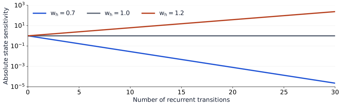
Longer paths multiply more derivatives

$$\frac{\partial h_T}{\partial h_s} =\prod_{t=s+1}^{T}\bigl[w_h\phi'(z_t)\bigr],\qquad s<T.$$

Vanishing: distant states barely influence the final state, weakening the learning signal.

Exploding: amplified sensitivities can produce very large gradients and unstable updates.

Plot: identity activation, so each factor is $w_h$. Vertical axis is logarithmic. State sensitivity is not the total shared-weight gradient. Pascanu, Mikolov & Bengio (2013).

Changing the activation changes the backward path

Activation $\phi(z)$	Local derivative	Consequence on a path
Identity $z$	$1$	Every factor is $w_h$
$\tanh(z)$	$1-\tanh^2(z)$	Saturation suppresses factors
ReLU $\max(0,z)$	$1$ for $z>0$; $0$ for $z<0$	An inactive unit blocks that path

ReLU is not differentiable at zero; implementations choose a convention there.

A different activation does not guarantee long-range learning.

Gradient clipping limits a large update signal. It cannot recover a signal that has vanished along a path.

Pascanu, Mikolov & Bengio (2013): On the difficulty of training recurrent neural networks.

Check one numerical backward step

Now choose $\phi=\tanh$, $(w_x,w_h,w_o)=(0.5,0.8,1)$, target $y=0.6$.
Illustrative inputs $(x_0,x_1,x_2)=(1,0.5,-0.5)$; fixed $h_{-1}=0$.

$t$	$z_t$	$h_t=\tanh(z_t)$
0	0.5	0.462
1	0.62	0.551
2	0.191	0.188

$\widehat y=0.188$, $L=0.0847$. What is $g_{z_2}$?

$$g_{z_2}=(\widehat y-y)w_o(1-h_2^2) \approx(-0.412)(1)(0.964)=-0.397.$$

Full backward ledger · Code replay / play · Continue to probability

Values rounded for display; checked at full precision against autograd and finite differences. The half-squared-error loss uses the course symbol $L$ throughout this recap.

Part 1 · Probability describes the question

1. Probability
2. Likelihood
3. Bayesian inference
4. KL
5. VAE

Start with a joint table. Derive the rules. Extend them to continuous values.

Then ask what a distribution’s mean and spread tell us.

Reading route: Bishop, PRML, §1.2, then §§2.1–2.3. All examples and figures below are original course calculations.

Extra rain and independence questions are now optional practice. The distribution/moment bridge follows in four core frames; longer calculations are optional practice. Say the loss-to-probability transition aloud: we know how to differentiate this loss; we will next explain where it comes from.

Outcomes, events, and random variables

One observation: a day with two binary values.

$R$: rain, $0$ = dry, $1$ = rain.
$S$: signal, $0$ = absent, $1$ = present.

$$\Omega=\{(0,0),(0,1),(1,0),(1,1)\}.$$

Outcome: one pair, such as $(1,1)$.

Event: all outcomes with rain.

$$A=\{(1,0),(1,1)\}=\{R=1\}.$$

Random variable: $R$ assigns 0 or 1 to each outcome.

A probability assigns weight to an event.

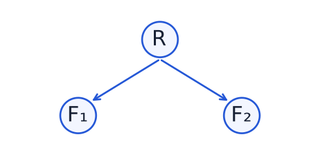
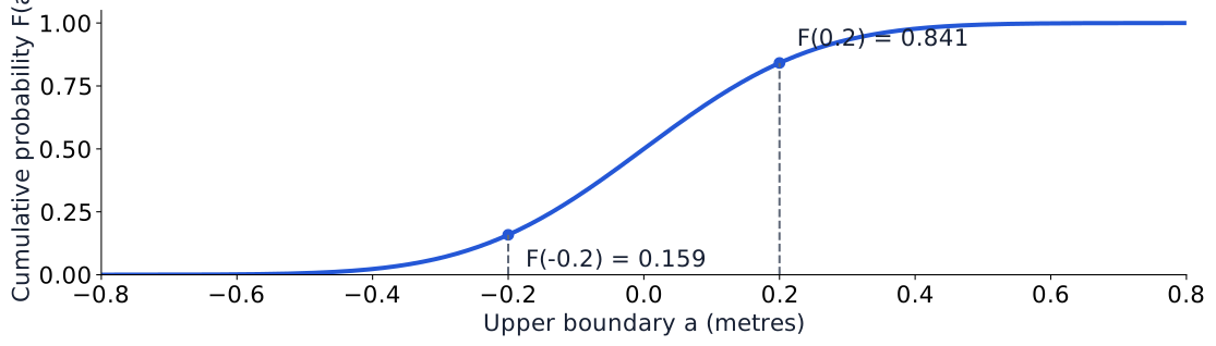
Synthetic teaching example. Real data need a rain threshold and signal definition. $P(A)\ge0$, $P(\Omega)=1$; disjoint events add. Bishop, PRML, §1.2.

A count table records both variables

100 synthetic outcomes. Here $Y=R$ (rows) and $X=S$ (columns).

$Y\backslash X$	$x_0$	$x_1$	Row total
$y_0$	54$n_{00}$	6$n_{01}$	60$r_0$
$y_1$	16$n_{10}$	24$n_{11}$	40$r_1$
Column total	70$c_0$	30$c_1$	100$N$

Cell count: $n_{ij}$

Column total: $c_j=\sum_i n_{ij}$
Row total: $r_i=\sum_j n_{ij}$

Grand total: $N=\sum_{i,j}n_{ij}$

$$\widehat p_N(y_i,x_j)=\frac{n_{ij}}{N}.$$

Highlighted joint event:

$$\widehat p_N(R=1,S=1)=\frac{24}{100}.$$

Joint means that both conditions hold in the same observation.

$\widehat p_N$: empirical proportions. Uniform sampling from this finite table gives these probabilities exactly. Population probabilities require a sampling model. Original editable table inspired by Bishop, PRML §1.2.

Conditioning changes the denominator

Keep the highlighted event $Y=y_1$ and $X=x_1$. Change the reference group.

$Y\backslash X$	$x_0$	$x_1$	Row total
$y_0$	54$n_{00}$	6$n_{01}$	60$r_0$
$y_1$	16$n_{10}$	24$n_{11}$	40$r_1$
Column total	70$c_0$	30$c_1$	100$N$

Joint: both conditions, among all $N$.

$$\widehat p_N(y_i,x_j)=\frac{n_{ij}}{N}.$$

Marginal: any row, in column $j$.

$$\widehat p_N(x_j)=\frac{\sum_i n_{ij}}{N}=\frac{c_j}{N}.$$

Conditional: row $i$, among column $j$.

$$\widehat p_N(y_i\mid x_j)=\frac{n_{ij}}{c_j},\qquad c_j>0.$$

$\widehat p_N(R=1\mid S=1)=24/30=0.8$: retain the signal column, then normalize.

For iid trials, as $N\to\infty$, empirical proportions converge to population probabilities (with positive conditioning probability). The probability rules themselves are exact identities. Bishop, PRML §1.2.

Sum and product rules follow from the counts

Write $p(y_i,x_j)$ for $P(Y=y_i,X=x_j)$. The same rules hold beyond this table.

$Y\backslash X$	$x_0$	$x_1$	Row total
$y_0$	54$n_{00}$	6$n_{01}$	60$r_0$
$y_1$	16$n_{10}$	24$n_{11}$	40$r_1$
Column total	70$c_0$	30$c_1$	100$N$

Sum rule: gather every row in column $j$.

$$p(x_j)=\sum_i p(y_i,x_j).$$

Product rule: split the cell’s fraction.

$$\frac{n_{ij}}{N}=\frac{n_{ij}}{c_j}\frac{c_j}{N}.$$

$$p(y_i,x_j)=p(y_i\mid x_j)p(x_j).$$

Sum out a variable. Factor the joint by conditioning on a variable.

The count identity is exact for finite-table sampling, with $c_j>0$. General probability identities: Bishop, PRML §1.2. Extra calculations and questions.

Bayes reverses the conditioning

The same joint event has two factorizations. Hold $i,j$ fixed.

$Y\backslash X$	$x_0$	$x_1$	Row total
$y_0$	54$n_{00}$	6$n_{01}$	60$r_0$
$y_1$	16$n_{10}$	24$n_{11}$	40$r_1$
Column total	70$c_0$	30$c_1$	100$N$

$$\begin{aligned} p(y_i,x_j)&=p(y_i\mid x_j)p(x_j)\\ &=p(x_j\mid y_i)p(y_i). \end{aligned}$$

Divide by $p(x_j)$ and apply the sum rule to the evidence.

$$p(y_i\mid x_j)=\frac{\overbrace{p(x_j\mid y_i)}^{\text{likelihood}}\overbrace{p(y_i)}^{\text{prior}}} {\underbrace{\sum_k p(x_j\mid y_k)p(y_k)}_{\text{evidence }p(x_j)}}.$$

Require $p(x_j)>0$. The sum covers all disjoint, exhaustive $Y$ categories. Joint symmetry exchanges variable order; conditional probabilities answer different questions. Bishop, PRML §1.2.

Steve: librarian or farmer?

Steve is reserved, helpful, orderly, and attentive to detail.

Which seems more likely: Steve is a librarian, or Steve is a farmer?

Imagine sampling him uniformly from a population containing only these two occupations. Commit to an intuition before seeing the counts.

What information is missing? The occupation proportions and how often the description occurs within each occupation.

Adapted from 3Blue1Brown’s original Steve problem. Open the original page for its visual explanation, or continue with the local worked example.

Steve: condition on the observed evidence

Teaching population: 10 librarians (40% shy), 200 farmers (10% shy).
Use Shy as the simplified evidence category; Not shy is its complement.

Occupation	Shy	Not shy	Total
Librarian	4	6	10
Farmer	20	180	200
Total	24	186	210

Find $P(\mathrm{Shy}\mid\mathrm{Lib})$, $P(\mathrm{Shy}\mid\mathrm{Farm})$, $P(\mathrm{Lib})$, and $P(\mathrm{Farm})$.

$P(\mathrm{Shy}\mid\mathrm{Lib})=0.4$, $P(\mathrm{Shy}\mid\mathrm{Farm})=0.1$;
$P(\mathrm{Lib})=10/210=1/21$, $P(\mathrm{Farm})=200/210=20/21$.

$$P(\mathrm{Lib}\mid\mathrm{Shy})= \frac{0.4(1/21)}{0.4(1/21)+0.1(20/21)} =\frac{4}{24}=\frac16\approx16.7\%.$$

Librarian probability rises from $1/21$ to $1/6$; farmer probability is still $5/6$.

Assumed counts, not measured occupation/personality statistics. 3Blue1Brown · Probability practice.

Bernoulli: a distribution over a binary observation

$R$ is a binary observation; $r$ is its probability of success.
$R\sim\operatorname{Bernoulli}(r)$ means “$R$ has a Bernoulli distribution,” $0\le r\le1$.

$$P(R=0)=1-r,\qquad P(R=1)=r.$$

Does changing $r$ change the possible outcomes or their weights?

It changes their weights. At $r=0$ or $r=1$, one outcome has all the mass.

The symbol $\sim$ means “distributed as.” A single observation is still 0 or 1. Bishop, PRML §2.1.

Expectation and variance

Expectation: probability-weighted average.

$$\mu=\mathbb E[X]=\sum_x xP(X=x).$$

Variance: average squared deviation.

$$\operatorname{Var}(X)=\mathbb E[(X-\mu)^2].$$

For Bernoulli: $\mathbb E[R]=0(1-r)+1r=r$, $\operatorname{Var}(R)=r(1-r)$.

Do equal means imply equal variances?

No: these plots have the same centre and different spread.

$X$: random variable; $x$: a possible value. Standard deviation $\operatorname{SD}(X)=\sqrt{\operatorname{Var}(X)}$ has the original units; variance has squared units. Bishop, PRML, Section 1.2.2.

For any quantity f(X), E[f(X)] = sum_x f(x)P(X=x). With finite second moments, Var(X)=E[X²]−E[X]². A Bernoulli mean of 0.5 does not make 0.5 a possible individual observation. Variance is zero at r=0 or r=1.

Continuous probability is area under a density

A normal (Gaussian) distribution is a bell-shaped density.
$X\sim\mathcal N(\mu,\sigma^2)$: mean $\mu=0$ m; standard deviation $\sigma=0.2$ m; variance $\sigma^2$.
$p_X(x)$ is the density of $X$ at a possible value $x$.

$$P(a\le X\le b)=\int_a^b p_X(x)\,dx,\qquad \int p_X(x)\,dx=1.$$

Continuous weighted average: $\mathbb E[f(X)]=\int f(x)p_X(x)\,dx$; $f(X)$ is the quantity averaged.

Density at 0 m is about 1.99 per metre. What is $P(X=0)$?

$P(X=0)=0$. An interval has probability: $P(-0.2\le X\le0.2)\approx0.683$.

Density height has units 1/metre; probability is area. Gaussian density formula and location/scale · Bishop, PRML §§1.2.1, 2.3.

For expectation, take f(x)=x; for variance take f(x)=(x−mu)². Sum/integrate over support and assume the required moments exist. A density need not be below one. The Gaussian model is an assumption about measurement errors, not a consequence of a single Bernoulli observation.

The same rules use sums or integrals

$p_X(x)$: mass of $X=x$ (discrete), or density at $x$ (continuous).
Joint: describe $X,Y$ together. Marginal: retain $X$ by summing/integrating out $Y$.

Rule	Discrete	Continuous
Normalize $p\ge0$	$\sum_x p_X(x)=1$	$\int p_X(x)\,dx=1$
Eliminate $Y$	$p_X(x)=\sum_i p(x,y_i)$	$p_X(x)=\int p(x,y)\,dy$
Factor joint	$p(x,y)=p(x\mid y)p_Y(y)$	$p(x,y)=p(x\mid y)p_Y(y)$
Bayes	$p(y\mid x)=\dfrac{p(x\mid y)p_Y(y)}{\sum_k p(x\mid y_k)p_Y(y_k)}$	$p(y\mid x)=\dfrac{p(x\mid y)p_Y(y)}{\int p(x\mid v)p_Y(v)\,dv}$

The denominator totals every possible explanation of the observed $x$.

Condition where the marginal mass/density is positive. For densities, this defines conditioning even when a point has probability zero. General rules and practice. Bishop, PRML §§1.2–1.2.2.

Distinguish masses from densities and Gaussian modeling assumptions from justified approximation. Longer CDF, Beta, covariance and multivariable explanations are optional practice.

Part 2 · A probability model explains the loss

1. Probability
2. Likelihood
3. Bayesian inference
4. KL
5. VAE

Choose a distribution for observations.
Hold the observations fixed. Fit its parameters.

The negative log likelihood gives a loss.

The ordered rain sequence is synthetic and distinct from the joint table used in the probability recap. The tutorial also uses this synthetic fallback.

Observed data → likelihood → loss

Observed pairs $\mathcal D=\{(x_i,y_i)\}_{i=1}^n$; fit parameters $\theta$.
iid: independent, identically distributed pairs.

Joint dataset likelihood

$$p_\theta(\mathcal D)=\prod_i p_\theta(x_i,y_i).$$

Supervised: hold inputs fixed
Assume conditional independence:

$$p_\theta(y_{1:n}\mid x_{1:n})=\prod_i p_\theta(y_i\mid x_i).$$

Maximum likelihood estimation (MLE): maximize the conditional likelihood.

$$\widehat\theta_{\mathrm{MLE}} =\arg\max_\theta\prod_i p_\theta(y_i\mid x_i) =\arg\min_\theta\underbrace{-\sum_i\ln p_\theta(y_i\mid x_i)}_{L(\theta):\ \text{negative log likelihood (NLL)}}.$$

Loss recipe: support → model + assumptions → constrained outputs → NLL → sum/mean

Choose the observation model before choosing the loss.

$y_{1:n}=(y_1,\ldots,y_n)$. Natural-log loss is measured in nats. Mean NLL is $L/n$; omit only parameter-independent terms. $\arg\max/\arg\min$ selects maximizing/minimizing parameters. Bishop, PRML, Section 1.2.5.

The dataset likelihood is a joint distribution over observed pairs: for iid pairs p_theta(D)=product_i p_theta(x_i,y_i). Here iid means independent and identically distributed pairs. Using the product rule, it factors into p_theta(x_1:n) and p_theta(y_1:n|x_1:n). We directly choose a conditional model for supervised prediction. Dropping p_theta(X) from a joint objective would require it to be theta-independent. A shared conditional model can give different target distributions at different inputs; targets need not have identical marginals. Conditional independence is an assumption, not an identity. Taking negative logs turns the product into a negative sum and reverses maximization to minimization; the two expressions are equivalent optimization problems, not equal probability values. Sum and mean have the same unregularized optimum but different gradient scales.

Likelihood: fixed observations, variable parameters

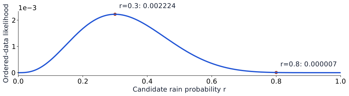
Synthetic ordered sequence $(1,0,0,1,0,0,0,1,0,0)$: 3 rain, 7 dry.
Assume independent, identically distributed (iid) Bernoulli observations with constant rain probability $r$.

$$\ell(r;\mathcal D)=p(\mathcal D\mid r)=\underbrace{r^3}_{\text{3 rain}}\underbrace{(1-r)^7}_{\text{7 dry}}.$$

Each rain contributes $r$; each dry day contributes $1-r$. Independence lets us multiply.

Fix the observations; vary $r$. The peak at $r=0.3$ is the MLE.

Likelihood scores the fixed data, not posterior uncertainty over $r$. Bishop, PRML, Section 1.2.3 and §2.1.

Observing only the count gives a binomial coefficient times r³(1−r)⁷; this parameter-independent factor leaves the MLE unchanged. The likelihood curve is not a normalized probability density over r.

Fixed Gaussian noise explains MSE

Real-valued target → Gaussian model → mean output → negative log

$$y_i\mid x_i,\theta\sim\mathcal N(\mu_\theta(x_i),\sigma^2),\qquad -\ln p_\theta(y_i\mid x_i)=\frac{(y_i-\mu_\theta(x_i))^2}{2\sigma^2}+\ln\sigma+\frac12\ln(2\pi).$$

Fixed common $\sigma>0$: the last two terms are constant in $\theta$. Mean NLL $=\mathrm{MSE}/(2\sigma^2)+\text{constant}$, where $\mathrm{MSE}=n^{-1}\sum_i(y_i-\mu_\theta(x_i))^2$.

MSE follows from a Gaussian model with fixed common observation variance.

Unequal fixed variances give weighted squared error. The RNN’s $\tfrac12(\widehat y-y)^2$ uses unit variance, omitting a constant. This noise assumption is not implied by the CLT. Bishop, PRML §1.2.5.

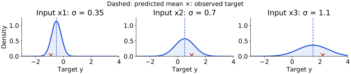
Input-dependent Gaussian noise

Real-valued target → Gaussian model → mean and log-variance outputs

$$s_i=s_\theta(x_i)=\ln\sigma_\theta^2(x_i),\qquad L_i=\frac12\left[e^{-s_i}(y_i-\mu_\theta(x_i))^2+s_i\right]+\frac12\ln(2\pi).$$

Derive this expression. Why must the $s_i$ term remain? Open the worked answer.

Increasing variance reduces the residual term; the log-variance term penalizes that inflation. Both outputs are fitted.

$s_i\in\mathbb R$ gives positive variance $e^{s_i}$. Heteroscedastic means input-dependent noise. With an exactly zero residual, unrestricted variance can collapse; constraints may be needed. Bishop, PRML §1.2.5.

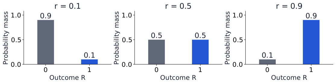
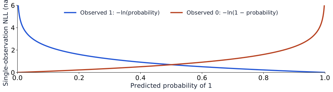
Bernoulli observations explain BCE

Binary target $y\in\{0,1\}$ → Bernoulli → logit $a_\theta(x)$ → $\pi=\operatorname{sigmoid}(a_\theta(x))$

$$p_\theta(y\mid x)=\pi^y(1-\pi)^{1-y} \quad\Rightarrow\quad L_i=-y\ln\pi-(1-y)\ln(1-\pi).$$

Both outcomes contribute through the same Bernoulli formula.

For the rain sequence: $L=-3\ln r-7\ln(1-r)$. Compute on logits for stability: PyTorch BCEWithLogitsLoss. Bishop, PRML §2.1.

Categorical observations explain multiclass CE

One class among $C$ → categorical → logits $a_c$ → $\pi_c=e^{a_c}/\sum_j e^{a_j}$

One-hot target $t_c\in\{0,1\}$, $\sum_c t_c=1$; class probabilities $\sum_c\pi_c=1$.

$$p_\theta(t\mid x)=\prod_{c=1}^C\pi_c^{t_c} \quad\Rightarrow\quad L_i=-\sum_{c=1}^C t_c\ln\pi_c=-\ln\pi_{\text{observed class}}.$$

Observed class: cat. Predicted probabilities: cat 0.7, dog 0.2, bird 0.1.
Which probabilities enter the loss?

Only the observed class: $L_i=-\ln(0.7)\approx0.357$ nats.
Multiple simultaneous binary labels instead need a Bernoulli model for each label.

The one-hot product describes one categorical draw; it does not assume independent classes. Use logits: PyTorch CrossEntropyLoss. Bishop, PRML §2.2.

The output head and observation model must agree

Observation model	Network output	Negative log likelihood
Gaussian, fixed common variance	Mean $\mu_\theta(x)$	Scaled squared error + constant
Gaussian, learned variance	Mean and log variance $s_\theta(x)$	Weighted residual + log-scale term
Bernoulli	One logit; sigmoid probability	BCE
Categorical	$C$ logits; softmax probabilities	Multiclass CE

Choose a model: temperature, rain/no rain, one handwritten digit class.

Temperature: Gaussian as an explicit assumption.
Rain/no rain: Bernoulli. One digit class: categorical.

A Gaussian assumption needs justification for the data. Sum or mean per-observation NLL consistently; regularization scaling matters later. Bishop, PRML §§1.2.5, 2.1–2.2.

Part 3 · Update uncertainty with evidence

1. Probability
2. Likelihood
3. Bayesian inference
4. KL
5. VAE

A prior describes uncertainty before these observations.
A posterior incorporates the observations.
Prediction carries the remaining uncertainty forward.

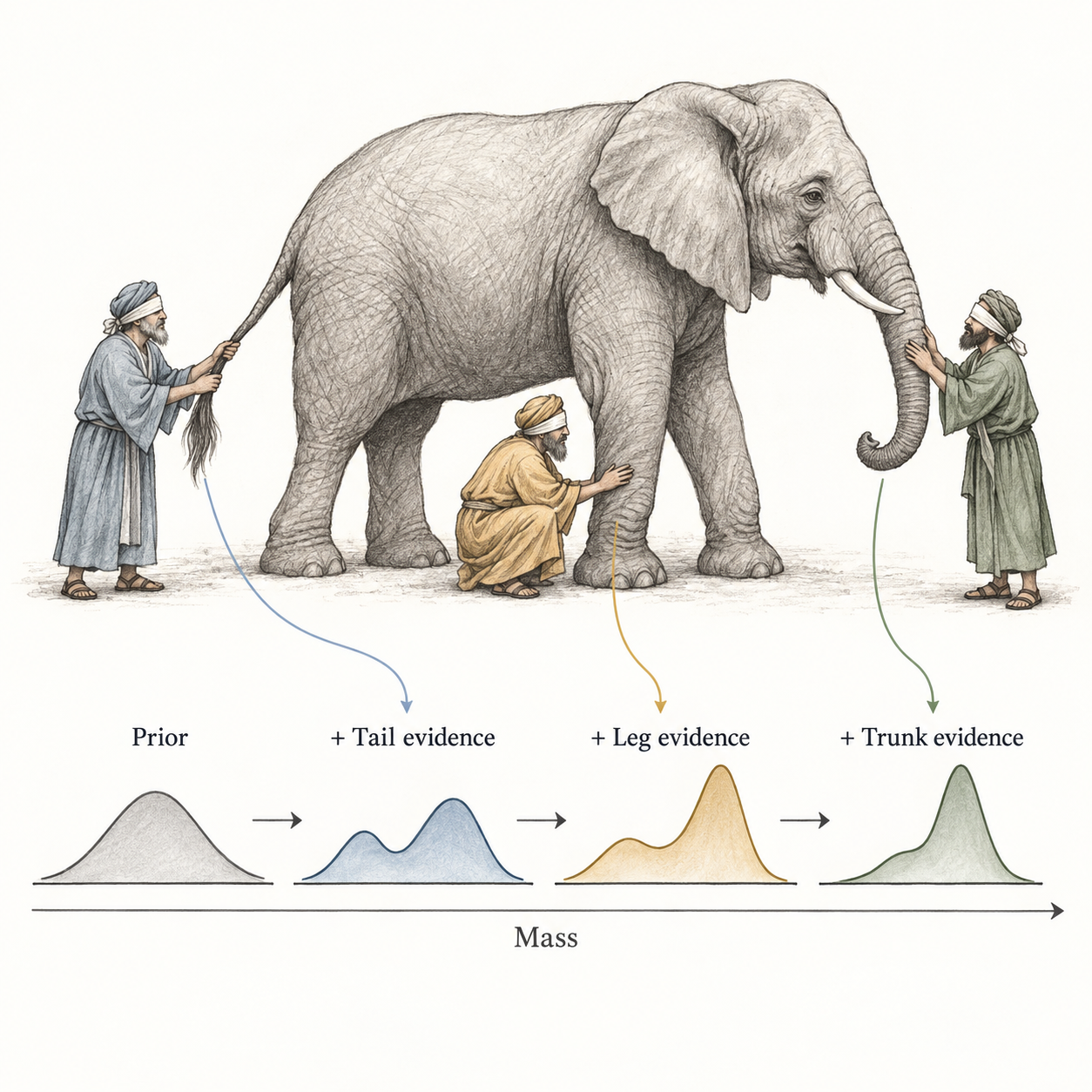
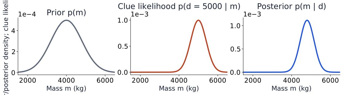
The elephant: a prior meets a noisy clue

Unknown mass $m\sim\mathcal N(4000,800^2)$ kg.
Hypothetical report $d=5000$ kg; observation model $d\mid m\sim\mathcal N(m,400^2)$.

$$p(\theta\mid\mathcal D)=\frac{p(\mathcal D\mid\theta)p(\theta)}{p(\mathcal D)}.$$

Multiply likelihood by prior, then normalize: here $m\mid d\sim\mathcal N(4800,358^2)$ approximately.

Hypothetical teaching values; exact posterior variance is 128000 kg². $\theta$ now denotes unknown model parameters; evidence integrates over them. The same rule updates a mass or network weights. Bishop, PRML §§1.2.3, 2.3.6.

The elephant: update one clue at a time

$m$: unknown mass.
$e_1,e_2,e_3$: tail, leg, trunk clues.

Start: $p_0(m)=p(m)$.

Tail: $$p_1(m)\propto p(e_1\mid m)p_0(m).$$

Leg: $$p_2(m)\propto p(e_2\mid m,e_1)p_1(m).$$

Trunk: $$p_3(m)\propto p(e_3\mid m,e_1,e_2)p_2(m).$$

Normalize each curve to area one. This posterior becomes the next prior.

$\propto$ means “proportional to”: normalization is omitted. Instructor-supplied conceptual illustration, not computed posteriors. Bishop, PRML, Section 1.2.3.

Each likelihood needs an assumed observation model connecting the clue to mass; the picture does not specify such models or numerical data. Conditional likelihoods retain earlier clues, avoiding an unstated conditional-independence assumption. Curves illustrate successive beliefs, not separate distributions of tail/leg/trunk measurements. New evidence need not reduce uncertainty at every step. The numerical example on the preceding slide is a different, explicitly specified Gaussian observation model.

MLE, MAP, and a full posterior

Result	Operation	What do we keep?
MLE — maximum likelihood estimation	Maximize $p(\mathcal D\mid\theta)$	One parameter setting at the likelihood peak
MAP — maximum a posteriori estimation	Maximize $p(\theta\mid\mathcal D)$	One parameter setting at the posterior-density peak (mode)
Full posterior	Normalize $p(\mathcal D\mid\theta)p(\theta)$	Entire distribution: spread and possible multiple modes

Does a MAP neural network retain uncertainty over its weights?

It keeps one setting. The full posterior retains how uncertainty is distributed.

An estimate locates a peak; a distribution also describes the remaining spread.

Compare approaches · Rainfall example. Bishop, PRML, Section 1.2.3 (one subsection).

MLE and MAP can have multiple maximizers; the table describes choosing one. Neither method alone stores the posterior. Frequentist uncertainty analysis can accompany a point estimator; the comparison is not “frequentists cannot quantify uncertainty.” MAP means maximum a posteriori, not a posterior mean.

Gaussian weight prior and quadratic penalty

Task: fit the data while expressing a preference for weights near zero.
Assume independent $\theta_j\sim\mathcal N(0,\tau^2)$; fixed $\tau$ is the prior standard deviation.

$$p(\theta_j)=\frac{1}{\sqrt{2\pi\tau^2}}\exp\!\left(-\frac{\theta_j^2}{2\tau^2}\right) \quad\Rightarrow\quad -\ln p(\theta_j)=\frac{\theta_j^2}{2\tau^2}+\text{constant}.$$

Sum over independent weights: $-\ln p(\theta)=\|\theta\|_2^2/(2\tau^2)+\text{constant}$, where $\|\theta\|_2^2=\sum_j\theta_j^2$.

Narrower prior (left) → steeper quadratic penalty (right).

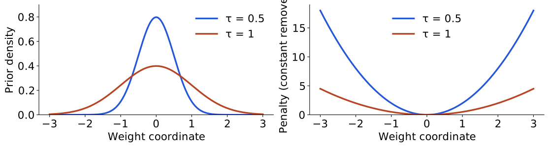
$\tau$: weight-prior scale; $\sigma$: observation-noise scale. The next slide combines this penalty with NLL through MAP. Bishop, PRML, Section 1.2.6.

This is the Gaussian density already encountered, now applied to an unknown weight rather than observation noise. There is no additional Gaussian theorem. Independence makes the joint prior a product; logarithms turn that product into a sum. The normalization is constant in theta because tau is fixed. Equivalently p(theta) is proportional to exp(−||theta||²/(2tau²)); propto is “proportional to,” not alpha. State explicitly whether biases are included when implementing this interpretation.

MAP produces L2 regularization

Extend the loss recipe: observation NLL + negative log prior → MAP

$$\widehat\theta_{\mathrm{MAP}} =\arg\min_\theta\left[-\ln p(\mathcal D\mid\theta)-\ln p(\theta)\right].$$

$$=\arg\min_\theta\left[\sum_{i=1}^n L_i(\theta)+\frac{\|\theta\|_2^2}{2\tau^2}\right].$$

Written objective	Coefficient giving this MAP fit
Mean NLL $+\lambda\|\theta\|_2^2$	$\lambda=1/(2n\tau^2)$
MSE $+\lambda\|\theta\|_2^2$	$\lambda=\sigma^2/(n\tau^2)$

The L2 coefficient depends on the loss scale and reduction.

Drop evidence, which is constant in $\theta$. MSE row assumes fixed common Gaussian variance $\sigma^2$, with no factor ½ in MSE. MAP is point estimation; decoupled optimizer weight decay is not generally this objective. Bishop, PRML §1.2.6.

Prediction after fitting

One fitted parameter setting

$$p_{\widehat\theta_{\mathrm{MAP}}}(y_*\mid x_*).$$

Evaluate one model at the new input.

Posterior predictive

$$\int p_\theta(y_*\mid x_*)p(\theta\mid\mathcal D)\,d\theta.$$

Average predictions over parameter uncertainty.

Does a stronger L2 penalty guarantee better validation predictions?

No. It changes the tradeoff with data fit; validation performance depends on the model and data.

L2 supplies a MAP objective; it does not perform posterior averaging.

$x_*,y_*$ denote a future input and target. Rainfall prediction. Bishop, PRML §§1.2.3, 2.1.1.

Frequentist and Bayesian approaches to ML

Question	Frequentist approach	Bayesian approach
Unknown parameters	Fixed but unknown	Uncertainty represented by prior/posterior
Use of evidence	Sampling model; MLE is one example	Likelihood × prior, then normalize
Report uncertainty	Repeated-sampling properties of procedures	Posterior and posterior predictive distributions
Prediction here	Evaluate a fitted model	Average over posterior; MAP retains one mode
Modern AI connection	Neural regression/classification; next-token NLL	Bayesian neural networks; approximate latent inference in VAEs

Both quantify uncertainty. NLL is shared machinery.

VAE here: approximate posterior over codes; fitted network weights. Bishop, PRML, Section 1.2.3 · Kingma & Welling, §§2–3. Return to estimates.

In frequentist inference, the unknown parameter is fixed. Repeating data collection and fitting would produce different estimates; uncertainty statements concern that repeated-sampling behavior. Bayesian inference conditions on the observed dataset and represents uncertainty about the parameter with a posterior. For rainfall, MLE selects r=3/10, while the Bayesian update retains a distribution over possible r values. The comparison concerns interpretations and procedures, not whether one approach has enough data or is universally better. MLE is not the whole frequentist framework, and MAP is not full posterior inference. A frequentist procedure can quantify uncertainty; a Bayesian procedure can report a point decision. Likelihood/NLL objectives also occur in Bayesian inference, so using a familiar neural loss does not by itself settle the philosophical interpretation. Next-token prediction uses a categorical observation model. The VAE applies Bayes and approximate inference to per-image latent variables, while encoder/decoder weights are point estimates in this lecture.

Part 4 · Compare distributions

1. Probability
2. Likelihood
3. Bayesian inference
4. KL
5. VAE

Score the same outcomes with two distributions.
KL measures the average extra log loss relative to a reference.

Bishop, PRML, §§1.6–1.6.1. Natural logarithms and nats throughout this lecture.

Standalone information theory is deferred. The exact two-state toy below is discrete and explicitly illustrative; the later VAE has continuous latent coordinates. Do not imply a trained VAE or apply the Gaussian reparameterization formula to the discrete toy.

KL measures average extra log loss

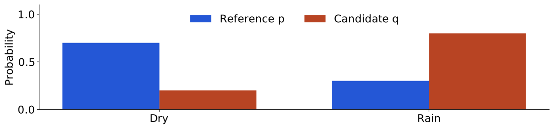
Dry/rain reference frequencies: $p=(0.7,0.3)$.
Candidate predictions: $q=(0.2,0.8)$. Average outcomes using $p$.

For outcome $a$, score with $q$: $-\ln q(a)$; reference score: $-\ln p(a)$.
Extra log loss: $-\ln q(a)-[-\ln p(a)]=\ln[p(a)/q(a)]$.

$$\operatorname{KL}(p\Vert q)=\sum_a p(a)\ln\frac{p(a)}{q(a)}\approx0.583\ \text{nats}.$$

The first argument supplies the averaging weights.

$a$: dry or rain. Nats: units of log loss using natural logs. Here $p$ is empirical, not a known population law. Bishop, PRML, Section 1.6.1.

The formula compares expected log losses under the same reference distribution. Individual outcomes can have negative extra loss, but the weighted total is nonnegative. The candidate is not used as the averaging distribution in KL(p||q).

KL has a direction

Expression	Average under	Value
$\operatorname{KL}(p\Vert q)$	$p=(0.7,0.3)$	0.583 nats
$\operatorname{KL}(q\Vert p)$	$q=(0.2,0.8)$	0.534 nats
$\operatorname{KL}(p\Vert p)$	$p$	0

KL is nonnegative; individual summands can be negative.
If $p(a)>0$ but $q(a)=0$, the forward KL is infinite.

For densities: $\operatorname{KL}(p\Vert q)=\int p(u)\ln[p(u)/q(u)]\,du$.

KL is a divergence, not a distance metric.

Zero means agreement almost everywhere; appropriate support and finite terms are assumed. KL is asymmetric and need not satisfy the triangle inequality. Bishop, PRML §1.6.1.

Part 5 · Infer and generate with a VAE

1. Probability
2. Likelihood
3. Bayesian inference
4. KL
5. VAE

A latent code is a small vector of hidden coordinates.
First specify how this code can generate an observation.
Then ask which codes could explain an observed image.
Approximate that inverse problem with a trainable distribution.

Kingma & Welling, Auto-Encoding Variational Bayes, §§2.1–2.2. Generative and inference routes are developed before the full architecture.

AE and VAE: point code or distribution

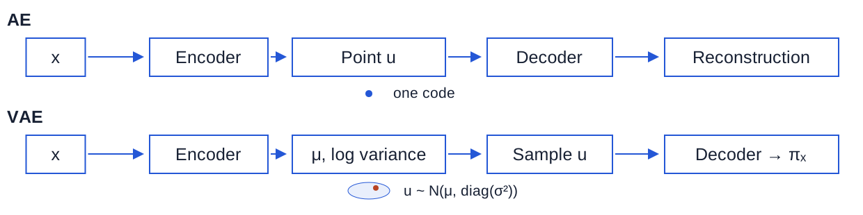
AE: encoder returns a point.
Reconstruction alone does not specify a prior for generating new codes.

VAE: encoder returns Gaussian parameters.
The generative model also specifies $p(u)$ and $p_\theta(x\mid u)$.

The VAE learns an approximate distribution of plausible codes for each image.

$x$: image; $u$: latent coordinate vector; $\theta$: decoder weights; $\psi$: encoder weights. Paper $z,\phi$ become course $u,\psi$; course $\phi$ remains an activation. Kingma & Welling, §§2–3.

Generation and inference

$$p_\theta(x,u)=p(u)p_\theta(x\mid u).$$

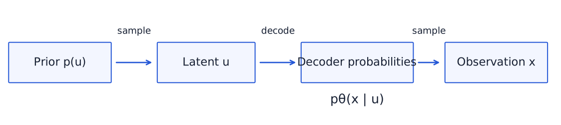
Generate: $u\sim p(u)$, then $x\sim p_\theta(x\mid u)$.

Infer: given $x$, find plausible $u$ using $p_\theta(u\mid x)$.

The encoder approximates inference; the prior and decoder define generation.

Network weights are point estimates here. Per-image latent uncertainty is not a Bayesian posterior over those weights. Kingma & Welling, §2.1.

Bayes for a two-pixel image

Prior $p(u=0)=p(u=1)=0.5$; pixels are independent given the code.

Code	$p(x_1=1\mid u)$	$p(x_2=1\mid u)$	$p((1,0)\mid u)$
$u=0$	0.8	0.2	$0.8(1-0.2)=0.64$
$u=1$	0.3	0.7	$0.3(1-0.7)=0.09$

$$p(x=(1,0))=0.5(0.64)+0.5(0.09)=0.365.$$ $$p(u\mid x)=\frac{p(x\mid u)p(u)}{p(x)}=(64/73,9/73)\approx(0.877,0.123).$$

Same Bayes rule as Steve: replace occupations with candidate codes.

Exact discrete teaching model, not a continuous VAE or a trained encoder. All four images normalize under each code. Check exact ELBO arithmetic.

The posterior needs an evidence integral

For continuous codes, use a spherical standard-normal prior:
independent $u_1,u_2\sim\mathcal N(0,1)$, written $u\sim\mathcal N(0,I_2)$.
Covariance averages the product of two variables’ deviations from their means.
$I_2$ is the identity covariance: unit variance in each coordinate and zero covariance between them.

$$p_\theta(u\mid x)=\frac{p_\theta(x\mid u)p(u)}{\underbrace{\int p_\theta(x\mid v)p(v)\,dv}_{p_\theta(x)}}.$$

At one code

The decoder can evaluate $p_\theta(x\mid u)$.

Across all codes

Many codes can explain one image. A nonlinear decoder can make this integral impractical.

Evidence averages over all possible codes, not just one decoder evaluation.

Spherical means equal spread in every direction. $v$ is a dummy integration variable. Continuous variables alone do not imply intractability; model structure matters. Kingma & Welling, §2.1; Bishop, PRML §10.1.

The encoder proposes an approximate posterior

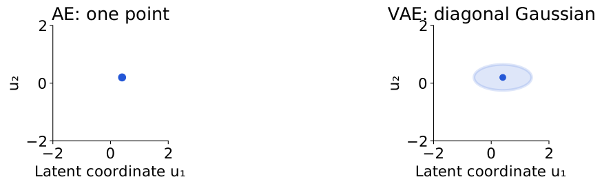
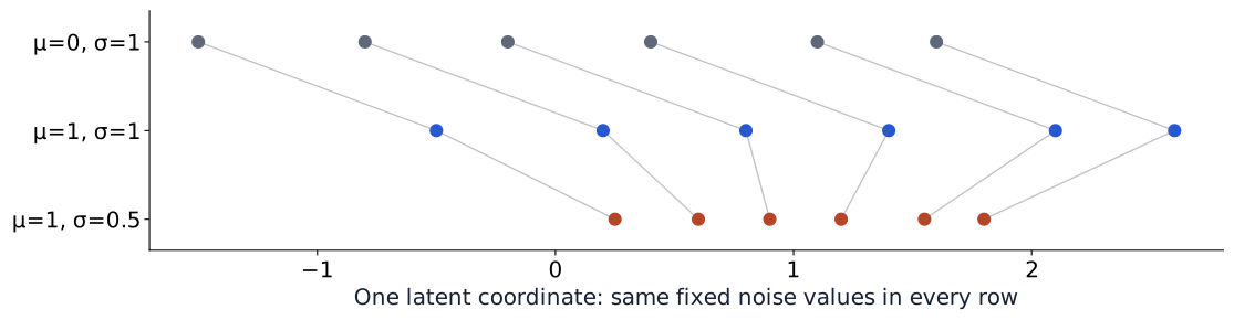
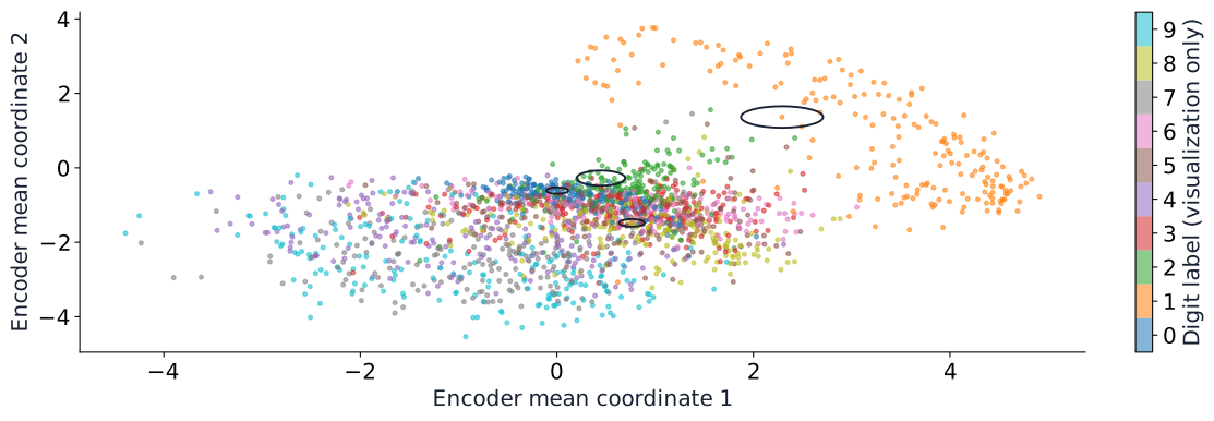
Given $x$, the encoder predicts centre $\mu_u(x)$ and spreads $\sigma_u(x)$.
Under $q$, the two coordinates are independent:

$$u_j\mid x\sim\mathcal N(\mu_{u,j}(x),\sigma_{u,j}^2(x)),\qquad j=1,2.$$

Different coordinate spreads → an axis-aligned ellipse; equal spreads → a circle.

$$q_\psi(u\mid x)=\mathcal N\!\left(\mu_u(x),\operatorname{diag}(\sigma_u^2(x))\right).$$

$\operatorname{diag}$: coordinate variances on the diagonal; zeros elsewhere.

Encoder outputs $\mu_u$ and $\mathrm{logvar}_u=\ln\sigma_u^2$; $\sigma_u=\exp(\tfrac12\mathrm{logvar}_u)$. Covariance practice. Kingma & Welling, §3.

The prior is spherical, but the encoder approximation has separate coordinate variances for each image. Its covariance is diagonal: zero cross-coordinate covariance implies independence for this Gaussian family. In general, zero covariance does not imply independence. A spherical approximate posterior is possible but imposes equal spreads; keep the existing diagonal model. A single diagonal Gaussian cannot capture correlated or multimodal posterior structure. The ellipse depicts coordinate standard deviations, not a calibrated confidence region. Reuse one encoder across images; psi denotes its fitted weights.

Bayes explains the ELBO

We need a training objective even when the exact latent posterior is hard to compute.
$q=q_\psi(u\mid x)$ is the encoder’s approximation; $\mathbb E_q$ averages over its possible codes.

$$\ln p_\theta(x)=\underbrace{\mathcal E}_{\text{evidence lower bound (ELBO)}} +\underbrace{\operatorname{KL}(q\Vert p_\theta(u\mid x))}_{\text{nonnegative posterior gap}}.$$

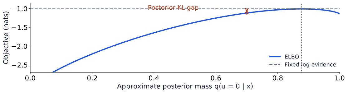
Bayes and the definition of KL give a usable expression:

$$\mathcal E=\mathbb E_q[\ln p_\theta(x,u)-\ln q_\psi(u\mid x)].$$

Log evidence $\ln p_\theta(x)$:
how well the generative model explains $x$ after averaging over the prior.

Posterior gap:
how far the encoder’s $q$ is from the exact posterior.

The gap cannot be negative: $\mathcal E\le\ln p_\theta(x)$.

Matching the exact posterior makes the bound exact. Line-by-line derivation and return link. Kingma & Welling, §2.2.

Assume positive evidence, suitable support and finite terms. The identity comes from log p_theta(u|x)=log p_theta(x,u)−log p_theta(x), substituted into the KL definition. Evidence is constant in u, so it leaves the expectation. The linked derivation retains each algebraic step. This gap compares q to the exact posterior; the later computable objective contains a different KL, comparing q to the prior. The next slide holds the generative model fixed while changing q.

Tightening the lower bound

Hold the decoder and prior fixed. What changes when $q$ approaches the posterior?

The posterior gap shrinks and ELBO rises; evidence stays fixed.
Joint training also changes the generative model and its evidence.

The expected ELBO is bounded. One Monte Carlo estimate need not lie below log evidence. Exact numbers. Kingma & Welling, §2.2.

Two computable ELBO terms

Use the product rule $p_\theta(x,u)=p_\theta(x\mid u)p(u)$:

$$\mathcal E= \underbrace{\mathbb E_q[\ln p_\theta(x\mid u)]}_{\text{explain the observed image}} -\underbrace{\operatorname{KL}(q_\psi(u\mid x)\Vert p(u))}_{\text{compare to the prior}}.$$

If $q$ equals the exact posterior, must its KL to the prior be zero?

No. The posterior usually differs from the prior.
Posterior-gap KL: explains the bound. Prior KL: is subtracted inside ELBO.

Minimize $L_{\mathrm{VAE}}=-\mathcal E=$ reconstruction NLL $+$ prior KL.

These are different KL comparisons. We estimate reconstruction by sampling and compute the Gaussian prior KL analytically. Kingma & Welling, §2.2.

The reparameterization trick

Problem: how can reconstruction gradients pass through a random draw to the encoder?
Draw noise independently of the encoder, then transform it:

$$\epsilon\sim\mathcal N(0,I_2),\qquad u=\mu_u+\sigma_u\odot\epsilon.$$

Same noise: $\mu_u$ shifts samples; $\sigma_u$ changes spread.
Fix $\epsilon$ during backpropagation: $u$ is differentiable in both outputs.

Reconstruction gradient → sampled code → mean and spread → encoder weights.

$\odot$: coordinatewise multiplication. Sample fresh noise on later forward passes. Kingma & Welling, §2.4.

An opaque sampling operation does not expose the deterministic path for ordinary backpropagation. Reparameterization separates parameter-independent randomness from the differentiable transformation. For one fixed epsilon, partial u_j / partial mu_{u,j}=1 and partial u_j / partial logvar_{u,j}=sigma_{u,j} epsilon_j / 2. Standard deviation is exp(logvar/2). Autograd reaches both encoder heads through reconstruction, as it traced the RNN path; the analytic prior KL also supplies gradients. This is a pathwise estimator, not the only possible gradient estimator. Keeping epsilon fixed during one backward pass does not mean reusing the same draw forever.

The binary-image VAE loss

Thresholded MNIST: $x_j\in\{0,1\}$; decoder logits $a_{x,j}(u)$ give $\pi_{x,j}=\operatorname{sigmoid}(a_{x,j})$.

$$\underbrace{-\ln p_\theta(x\mid u)}_{\text{reconstruction NLL}} =-\sum_{j=1}^{784}[x_j\ln\pi_{x,j}+(1-x_j)\ln(1-\pi_{x,j})].$$

$$\underbrace{\operatorname{KL}(q_\psi\Vert\mathcal N(0,I))}_{\text{latent prior KL}} =\frac12\sum_{j=1}^{2}[\mu_{u,j}^2+\sigma_{u,j}^2-1-\ln\sigma_{u,j}^2].$$

Sum pixels and latent coordinates per image, then average images.
Standard VAE uses coefficient 1 on prior KL; $\beta_{\mathrm{VAE}}\ne1$ changes the objective.

Pixels conditionally independent given $u$; compute BCE on logits. Latent dimension is 2 in this pilot. Gaussian KL derivation · Implementation and pilot settings. Kingma & Welling, Appendices B/C.

Reconstruction: decode an observed image’s mean code

Mean code: the encoder’s two-coordinate centre $\mu_u(x)$.
$x\ \to\ \mu_u(x)\ \to\ \operatorname{decoder}\ \to\ \pi_x$ (pixel probabilities).

Top: original grayscale source. Middle: binary model input.
Bottom: each pixel’s predicted probability of being on, given the mean code.

A latent code is a coordinate vector; a probability image is the decoder’s mean output.

For a Bernoulli pixel, mean = probability of 1. Decode $\mu_u(x)$ for this deterministic display. Existing MNIST pilot: $\beta=1$; validation images; test set unused.

The bottom row is neither the original grayscale target nor sampled binary pixels. It is sigmoid(decoder(mu_u(x))). Decoding the mean code is not generally E_q[decoder(u)] because the decoder is nonlinear. Pilot: 12,000 train / 2,000 disjoint validation images; 15 epochs. The first validation example per label was selected before inspecting quality. Each displayed reconstruction uses its corresponding observed input.

A latent map shows what the encoder learned

Reading task: where does the encoder place each validation image?

One dot: one image’s mean code $\mu_u(x)$.
Axes: two learned latent coordinates.

Color: known digit label, used only for display.
Four ellipses: selected encoder distributions; semiaxes are one standard deviation.

Find an overlapping region. Class separation was not a training objective.

2,000 validation images, baseline $\beta=1$. Ellipses show model spread, not calibrated confidence. Original MNIST pilot.

Nearby codes can decode similarly, but the plot does not prove a unique meaning for either axis or measure classification quality. Colors were not supplied to the encoder during training. A dot summarizes only the distribution centre; the selected ellipses remind us that an encoder returns a distribution, not just a point. The pilot used 12,000 training images, 15 epochs; the official test set was unused.

Generate a new image from the prior

1. Draw a code: two independent standard-normal coordinates, $u\sim\mathcal N(0,I_2)$.
2. Decode probabilities: $\pi_x=\operatorname{sigmoid}(\operatorname{decoder}(u))$ for 784 pixels.
3. Sample an image: $x_j\sim\operatorname{Bernoulli}(\pi_{x,j})$ for each pixel.

Each column uses the same code: top = probabilities; bottom = sampled binary pixels.

Generation starts from a prior draw; reconstruction starts from an observed image.

No input image or encoder is needed for generation. $I_2$: unit coordinate variances, zero covariance. Baseline $\beta=1$, predeclared gallery; original pilot.

The spherical prior uses the same spread in every direction. Unlike reconstruction, this route does not infer a code from a selected input. The decoder’s probability image is its conditional mean under Bernoulli observations; actual sampled binary pixels may look noisy. Pixels are conditionally independent given u. Both rows share codes, but the second adds observation sampling. All predeclared draws are displayed, using the existing seeds. Larger KL weight adds prior pressure but does not guarantee better images.

One argument answers three questions

Question	Model-based answer
Why this loss?	Observation distribution → negative log likelihood
How does evidence change uncertainty?	Prior × likelihood → posterior → prediction
How can hidden causes explain an image?	Generative model → approximate latent posterior → ELBO → trainable encoder/decoder

Write the distribution, identify what is observed, and trace what is inferred or optimized.

Rainfall inference estimates a shared event probability.
This VAE infers a per-image code and optimizes shared network weights.
Compare frequentist and Bayesian approaches.

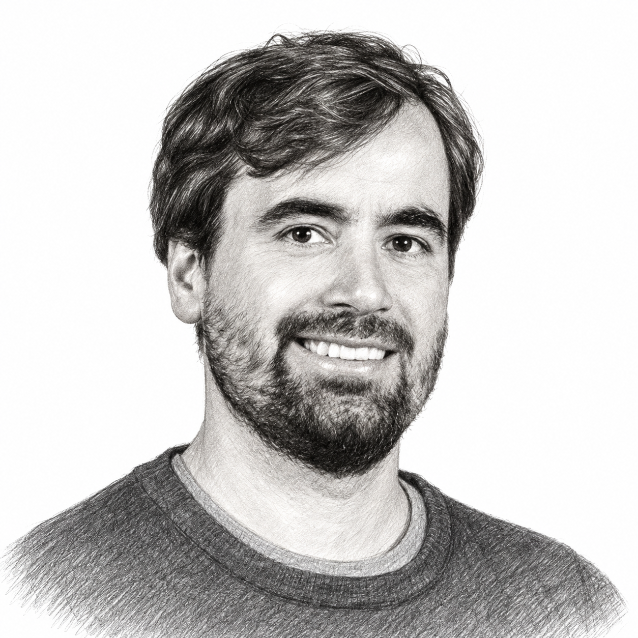
Person of the day: Diederik P. Kingma

Diederik P. (Durk) Kingma

• Coauthored Auto-Encoding Variational Bayes with Max Welling (2013 preprint).
• Coauthored Adam with Jimmy Ba (2014 preprint).
• PhD, University of Amsterdam, 2017, advised by Welling.

A learned inference network and a differentiable sampling path connect today’s probability model to neural-network training.

Kingma’s site · AEVB · Adam. Biography verified 2026-10-14. Portrait supplied by the instructor.

Kingma and Welling connect the generative model, learned inference network and reparameterized gradient estimator. Credit both authors when discussing AEVB.

Tutorial: predict, compute, and interpret

Rainfall

Same observations: likelihood → MLE → prior/posterior → prediction.
Explain which object describes data and which describes uncertainty about $r$.

VAE

Identify inferred codes and fitted weights.
Explain reconstruction, latent maps, generation, and the sampling gradient path.

State the model → predict → compute → explain.

Week 07 tutorial (draft) · Readable VAE core

The linked tutorial remains an educational draft and uses synthetic rainfall. Its real-weather extension requires explicit data choices; see the instructor publication record. Reserve time for students to explain predictions rather than only run cells. Discussion checkpoints: compare the same rainfall dataset across likelihood, MLE, posterior and prediction; explain assumptions behind MSE/BCE/CE and Gaussian-prior MAP/L2; identify inferred latent codes versus fitted weights and trace the reparameterization gradient path. Do not imply that MAP retains full posterior uncertainty.

Reading: gradients and probability

• Week 06 textbook: one scalar recurrent model. The accepted course derivation, notation, and diagrams.
• Pascanu, Mikolov & Bengio (2013). On the difficulty of training recurrent neural networks. ICML, PMLR 28(3), 1310–1318.
• Bishop (2006), Pattern Recognition and Machine Learning. Probability, likelihood and inference: §§1.2, 2.1, 2.3.6; information: §1.6; conditional independence: §8.2; VI: §10.1.

Reading: latent-variable inference

• Kingma & Welling, Auto-Encoding Variational Bayes (2013 preprint; ICLR 2014). §§2–3 and Appendices B/C: variational bound, reparameterization, Gaussian KL and observation models. Course notation translates paper $z,\phi$ to $u,\psi$, and paper ELBO $\mathcal L$ to course $\mathcal E$.
• Bishop, Pattern Recognition and Machine Learning (2006). §10.1: variational inference and the lower-bound decomposition.
• Torchvision MNIST. Dataset loading and train/test split. Pilot uses installed Torchvision 0.23.0 and PyTorch 2.8.0.

Elephant graphical abstract supplied by the instructor. RNN diagrams redraw the Week 06 model; diagrams and sensitivity plots are original course figures.

Optional depth begins here

The main lecture is complete. Use the following slides for practice or selected live derivations.

Open the practice menu.

Cross-entropy is entropy plus KL

$$H(p,q)=\mathbb E_p[-\ln q(A)] =\underbrace{H(p)}_{\mathbb E_p[-\ln p(A)]}+\operatorname{KL}(p\Vert q).$$

Our 7 dry and 3 rain observations define $\widehat p=(0.7,0.3)$:

$$\frac Ln=-0.7\ln0.2-0.3\ln0.8 \approx0.611+0.583\approx1.19\ \text{nats}.$$

When $p$ is fixed, which term changes as we fit $q$?

Only KL changes. Minimizing empirical categorical cross-entropy minimizes $\operatorname{KL}(\widehat p\Vert q)$. One-hot CE is $-\ln\pi_{\text{observed class}}$.

$H(p)$ is the fixed reference term. This exact finite discrete identity does not identify a continuous empirical measure with a density. Detailed information theory is deferred to later in the course. Bishop, PRML §1.6.1.

RNN practice: the full backward ledger

Same tanh example: $g_{z_t}=g_{h_t}(1-h_t^2)$, $g_{h_{t-1}}=w_hg_{z_t}$.

Backward order	$g_{h_t}$	$1-h_t^2$	$g_{z_t}$
$t=2$	−0.412	0.964	−0.397
$t=1$	−0.318	0.696	−0.221
$t=0$	−0.177	0.786	−0.139

Use these sensitivities to calculate all three parameter gradients.

$$\begin{aligned} \frac{\partial L}{\partial w_x}&=g_{z_0}(1)+g_{z_1}(0.5)+g_{z_2}(-0.5)\approx-0.0513,\\ \frac{\partial L}{\partial w_h}&=0+g_{z_1}h_0+g_{z_2}h_1\approx-0.321,\\ \frac{\partial L}{\partial w_o}&=(\widehat y-y)h_2\approx-0.0776. \end{aligned}$$

Calculate with full precision; displayed values are rounded. Return to checkpoint · Check with code.

Match the arithmetic to a short computation

import torch
w_x, w_h, w_o = [torch.tensor(v, dtype=torch.float64, requires_grad=True)
                 for v in [0.5, 0.8, 1.0]]
h = torch.tensor(0.0, dtype=torch.float64)
for x_t in [1.0, 0.5, -0.5]:
    h = torch.tanh(w_x * x_t + w_h * h)
prediction = w_o * h
loss = 0.5 * (prediction - 0.6) ** 2
loss.backward()
print([f"{w.grad.item():.3g}" for w in (w_x, w_h, w_o)])
# [-0.0513, -0.321, -0.0776]

Autograd follows the same dependencies we differentiated by hand.

Try changing one input or weight. Predict the gradient sign, then rerun.
Download the checked replay · Return to the checkpoint.

CPU only; requires PyTorch. Run python3 scalar-rnn.py. No training or dataset download.

Optional practice: probability

Use the same counts to check your reasoning. Each task has a worked answer revealed by a click.

1. Marginal and conditional probabilities
2. Weighted total probability
3. Independence and mutual exclusivity
4. Conditional independence

Public, ungraded lecture practice. Return to Steve · Continue with continuous probability.

Practice: marginal and conditional probabilities

	Signal absent	Signal present	Total
Dry	54	6	60
Rain	16	24	40
Total	70	30	100

Find $p(R=1)$, $p(S=1)$, $p(R=1\mid S=1)$, and $p(S=1\mid R=1)$. Which denominators change?

$$\begin{aligned} p(R=1)&=40/100=0.4, &p(S=1)&=30/100=0.3,\\ p(R=1\mid S=1)&=24/30=0.8, &p(S=1\mid R=1)&=24/40=0.6. \end{aligned}$$

Conditioning changes the reference group. The joint event is the same 24 observations; the two conditionals use different totals.

Normalized teaching counts; uniform sampling from the table. Bishop, PRML §1.2. Practice menu · Return to the denominator slide.

Practice: total probability uses group weights

Given the same table:

$$p(R=1\mid S=1)=\frac{24}{30},\quad p(R=1\mid S=0)=\frac{16}{70},\quad p(S=1)=0.3.$$

Recover $p(R=1)$. Why would an unweighted average of the two conditionals fail?

$$p(R=1)=\sum_{s\in\{0,1\}}p(R=1\mid S=s)p(S=s)$$ $$=\frac{24}{30}\frac{30}{100}+\frac{16}{70}\frac{70}{100}=0.4.$$

The groups contain 30 and 70 observations. Giving them equal weight would yield approximately $0.514$, describing a different sampling scheme.

The groups are disjoint and exhaustive. Combine sum and product rules. Bishop, PRML §1.2. Practice menu · Return to the rules.

Practice: independent or mutually exclusive?

$$R\perp S\ \Longleftrightarrow\ p(R=a,S=b)=p(R=a)p(S=b)\quad\text{for every }a,b.$$

Are rain and signal independent in our table? Can two mutually exclusive events with positive probability be independent?

Rain and signal: $p(R=1,S=1)=0.24$, whereas $p(R=1)p(S=1)=0.4(0.3)=0.12$. Independence fails.

Mutually exclusive events: their intersection has probability zero. If both have positive probability, their product is positive, so independence fails here too.

Independence means factorization. Mutual exclusivity means no shared outcomes.

One failed factorization disproves independence; checking one successful cell does not establish it in general. Bishop, PRML §1.2. Practice menu · Return to the rules.

Practice: independence after conditioning

A separate hypothetical sensor model

$$p(F_1,F_2\mid R)=p(F_1\mid R)p(F_2\mid R).$$

Each sensor has $p(F_i=1\mid R=1)=0.6$, $p(F_i=1\mid R=0)=0.1$; let $p(R=1)=0.4$.

Does conditional independence imply marginal independence? Compare $p(F_1=1,F_2=1)$ with $p(F_1=1)p(F_2=1)$.

$$p(F_i=1)=0.4(0.6)+0.6(0.1)=0.3;$$ $$p(F_1=1,F_2=1)=0.4(0.6)^2+0.6(0.1)^2=0.15\ne0.3^2.$$

No. Mixing groups with different signal rates induces marginal dependence in this model.

Factorization is a model assumption, not a conclusion from the first rain/signal table or a causal claim. Bishop, PRML §8.2. Practice menu · Return to Bayes.

Optional practice: distributions and moments

Explore the longer calculations. Each fixed question has a worked answer revealed by a click.

1. CDF and interval probability
2. Beta: a density over a probability
3. Covariance and dependence
4. Gaussian location and scale
5. When a normal approximation helps
6. Multivariable rules

Public, ungraded lecture practice. Return to the rules · Continue to likelihood.

The CDF accumulates probability up to a boundary

$$F_X(a)=P(X\le a)=\int_{-\infty}^{a}p_X(x)\,dx.$$

Use the two marked values to find $P(-0.2\le X\le0.2)$.

$$P(-0.2\le X\le0.2)=F_X(0.2)-F_X(-0.2)\approx0.683.$$

Rounded labels give 0.682; the full-precision calculation rounds to 0.683.

Same Gaussian as the core slide. $F_X'(x)=p_X(x)$ where differentiable. Bishop, PRML §1.2.1. Practice menu · Return to density.

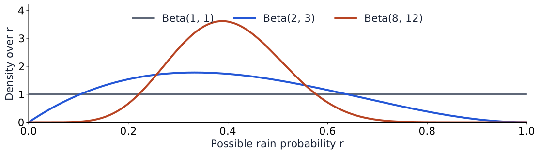
Beta: a density over a possible probability parameter

$$p(r)=\frac{r^{\alpha-1}(1-r)^{b_0-1}}{B(\alpha,b_0)},\qquad 0<r<1,\quad \alpha,b_0>0.$$

Do these curves describe a binary observation, or uncertainty over its probability $r$?

Uncertainty over $r$. The common mean is $\alpha/(\alpha+b_0)=0.4$ for Beta(2,3) and Beta(8,12); their variances are $0.04$ and about $0.0114$.

$B(\alpha,b_0)$ normalizes the density. These are example models, not successive updates. Bishop, PRML §2.1.1. Practice menu · Return to Bernoulli.

Covariance describes how two variables vary together

$$\operatorname{Cov}(X,Y)=\mathbb E[(X-\mathbb E[X])(Y-\mathbb E[Y])] =\mathbb E[XY]-\mathbb E[X]\mathbb E[Y].$$

The rain/signal table

$$\operatorname{Cov}(R,S)=0.24-(0.4)(0.3)=0.12.$$

Correlation divides by both standard deviations:

$$\operatorname{Corr}(R,S)=\frac{\operatorname{Cov}(R,S)}{\operatorname{SD}(R)\operatorname{SD}(S)}\approx0.535.$$

Does zero covariance guarantee independence?

No. Let $U$ be uniform on $\{-1,0,1\}$ and $V=U^2$.

$U$	−1	0	1
$V$	1	0	1

$\mathbb E[U]=\mathbb E[UV]=0$, so $\operatorname{Cov}(U,V)=0$. Yet $V$ is determined by $U$ and is not constant.

Finite second moments assumed. Correlation requires positive variances; independence implies zero covariance, but its converse fails in general. Bishop, PRML §1.2.2. Practice menu · Return to moments.

Gaussian: location and scale for continuous values

$$p_X(x)=\frac{1}{\sqrt{2\pi\sigma^2}}\exp\!\left[-\frac{(x-\mu)^2}{2\sigma^2}\right],\qquad \sigma>0.$$

Which parameter shifts the curve? Which parameter changes its width?

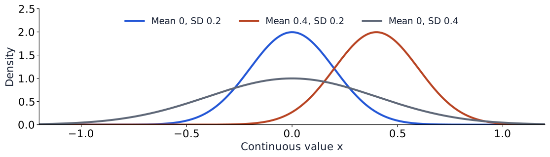
$\mu$ sets location; $\sigma$ sets spread. $\mathcal N(\mu,\sigma^2)$ has mean $\mu$ and variance $\sigma^2$. All these densities have unit area.

Gaussian support is the real line. Bishop, PRML §§1.2.4, 2.3. Practice menu · Return to density.

A normal approximation can help with counts

$K\sim\operatorname{Binomial}(n,r)$ counts $n$ independent Bernoulli($r$) trials, $0<r<1$.
Use $G\sim\mathcal N(nr,nr(1-r))$. Orange points show $P(k-0.5\le G\le k+0.5)$.

Why does the rare-event example make a poor approximation?

Normal approximation: Penn State STAT 414 §28.1. Accuracy depends on counts and the event; one trial stays binary. Gaussian regression noise requires a separate model assumption. Show worked answer · Practice menu.

Same moments, different count probabilities

Rare-event example: $K\sim\operatorname{Binomial}(20,0.02)$; $G\sim\mathcal N(0.4,0.392)$ is the matching Gaussian approximation.

Quantity	Binomial $K$	Gaussian $G$
Mean	0.4	0.4
Variance	0.392	0.392
Zero / zero bin	$P(K=0)\approx0.668$	$P(-0.5\le G\le0.5)\approx0.488$
Outside $[-0.5,20.5]$	0	About 7.53%

Only $nr=0.4$ successes are expected. The count law is skewed near zero; the Gaussian spreads too much probability beyond the bins for valid counts.

Matching mean and variance does not guarantee accurate count probabilities.

Original exact calculations; no renormalization of Gaussian bin probabilities. Return to comparison · Practice menu. Approximation method: Penn State STAT 414 §28.1.

Probability rules extend to many variables

Write $x_{1:m}=(x_1,\ldots,x_m)$, with $1\le m<k$. Shading marks the variables eliminated.

Marginalize the joint over every remaining coordinate

$p(x_{1:m})=$ $\sum_{x_{m+1},\ldots,x_k}$ $p(x_{1:k})$ (discrete)

$p(x_{1:m})=\int p(x_{1:k})$ $dx_{m+1}\cdots dx_k$ (continuous)

Chain rule: factor the joint in a chosen order

$$p(x_{1:m})=p(x_1)\prod_{j=2}^{m}p(x_j\mid x_{1:j-1}).$$

Does this factorization require independence?

No. The chain rule holds without independence; that extra assumption can simplify the conditionals.

Sum/integrate over each eliminated variable’s support. Mixed models combine sums and integrals. For $m=1$, the empty product is one. Bishop, PRML §§1.2, 8.2. Practice menu · Return to the rules.

Worked answer: input-dependent Gaussian loss

Start with the scalar Gaussian negative log density:

$$-\ln p(y_i\mid x_i)=\frac{(y_i-\mu_i)^2}{2\sigma_i^2}+\ln\sigma_i+\frac12\ln(2\pi).$$

Substitute $s_i=\ln\sigma_i^2$: $\sigma_i^{-2}=e^{-s_i}$ and $\ln\sigma_i=s_i/2$.

$$L_i=\frac12\left[e^{-s_i}(y_i-\mu_i)^2+s_i\right]+\frac12\ln(2\pi).$$

Writing $e_i=y_i-\mu_i$, $\partial L_i/\partial s_i=\tfrac12(1-e^{-s_i}e_i^2)$. For fixed nonzero residual, the optimum is $\sigma_i^2=e_i^2$. Without $s_i/2$, arbitrarily large variance drives the residual term toward zero.

The constant can be omitted; the fitted log-variance term cannot.

If $e_i=0$, $s_i\to-\infty$ drives this unrestricted NLL down without bound. This is observation noise, not a posterior over weights. Return to the question. Bishop, PRML §1.2.5.

Rainfall: the Beta prior gives an exact update

$$p(r)\propto r^{\alpha-1}(1-r)^{b_0-1},\qquad p(\mathcal D\mid r)=r^k(1-r)^{n-k}.$$

$$p(r\mid\mathcal D)\propto r^{\alpha+k-1}(1-r)^{b_0+n-k-1} \quad\Rightarrow\quad r\mid\mathcal D\sim\operatorname{Beta}(\alpha+k,b_0+n-k).$$

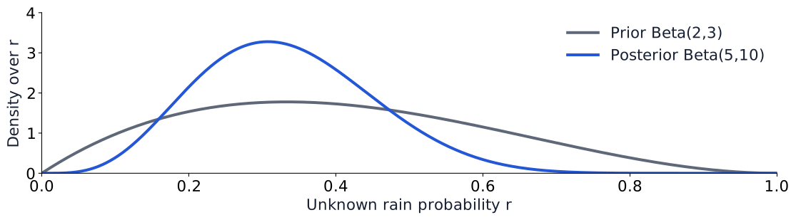
Beta(2,3) + 3 rain + 7 dry → Beta(5,10).

Conjugacy: the posterior remains in the prior’s distribution family. Constant $r$, common Bernoulli model, conditionally independent observations. Real weather may violate these assumptions. Bishop, PRML §2.1.1. Practice menu.

Same prior mean, different resistance to evidence

$$m_0=\frac{\alpha}{\alpha+b_0},\quad\kappa=\alpha+b_0, \qquad \mathbb E[r\mid\mathcal D] =\frac{\kappa}{\kappa+n}m_0+\frac{n}{\kappa+n}\frac{k}{n}.$$

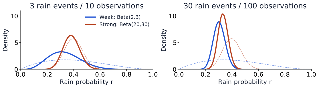
Change only $\kappa$: which posterior mean moves further toward $k/n=0.30$?

The weak prior moves farther: posterior mean 0.333 versus 0.383 after 3 of 10 rain observations.

Dashed = prior; solid = posterior. Synthetic datasets: $(n,k)=(10,3)$ and $(100,30)$. Fixed prior influence decreases in this model as $n$ grows. $n>0$ in the displayed weighted-average identity. Bishop, PRML §2.1.1. Practice menu.

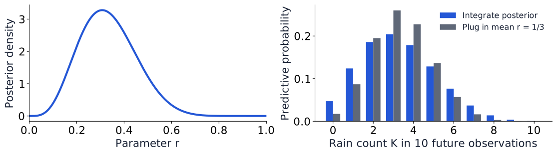
A posterior density is not a forecast of rain counts

Let $K$ count rain events in $q=10$ future observations.
Given $r$, use $K\mid r\sim\operatorname{Binomial}(q,r)$; retain the same model assumptions.

$$p(K=j\mid\mathcal D)=\int_0^1p(K=j\mid r)\,p(r\mid\mathcal D)\,dr.$$

Same mean count, different spread: integrating uncertainty changes the prediction.

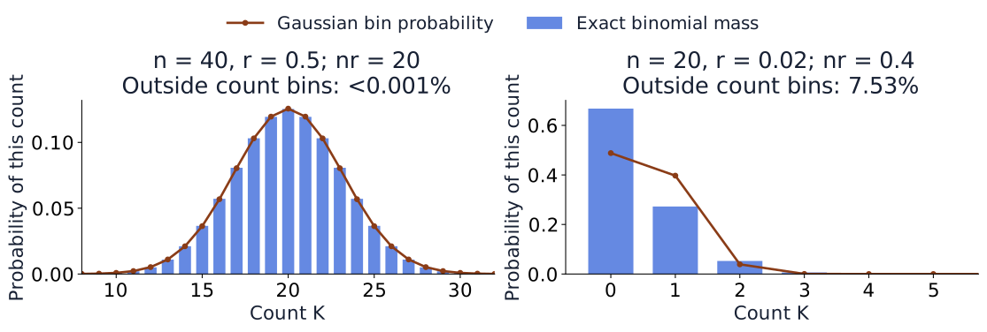
Beta-binomial variance $\approx3.47$; plug-in Binomial variance $\approx2.22$. Axes represent different variables and units. A credible interval for $r$ is not a prediction interval for $K$. Original calculation from the predictive integral; Bishop, PRML §2.1.1. Practice menu.

ELBO algebra from Bayes

For $q=q_\psi(u\mid x)$, insert Bayes into the definition of KL:

$$\begin{aligned} \operatorname{KL}(q\Vert p_\theta(u\mid x)) &=\mathbb E_q[\ln q-\ln p_\theta(u\mid x)]\\ &=\mathbb E_q[\ln q-\ln p_\theta(x,u)+\ln p_\theta(x)]\\ &=-\mathcal E+\ln p_\theta(x). \end{aligned}$$

Evidence does not depend on the code, so it leaves the expectation.
Rearrange: $\mathcal E=\ln p_\theta(x)-\operatorname{KL}(q\Vert\text{posterior})\le\ln p_\theta(x)$.

Appropriate support and finite expectations assumed. Return to ELBO. Kingma & Welling, §2.2.

Gaussian KL: take the expectation

For independent coordinates of $q=\mathcal N(\mu,\operatorname{diag}(\sigma^2))$, $p=\mathcal N(0,I)$:

$$\ln\frac{q(u)}{p(u)}=\frac12\sum_j\left[-\ln\sigma_j^2-\frac{(u_j-\mu_j)^2}{\sigma_j^2}+u_j^2\right].$$

Use $\mathbb E_q[(u_j-\mu_j)^2]=\sigma_j^2$ and $\mathbb E_q[u_j^2]=\mu_j^2+\sigma_j^2$:

$$\operatorname{KL}(q\Vert p)=\frac12\sum_j[\mu_j^2+\sigma_j^2-1-\ln\sigma_j^2].$$

Each coordinate’s contribution is zero at $\mu_j=0$, $\sigma_j^2=1$.

This is KL to the prior, not to the model posterior. Return to image loss. Kingma & Welling, Appendix B.

Check the signs with the exact toy

For $x=(1,0)$ and $q(u\mid x)=(0.7,0.3)$:

Quantity	Calculation	Nats
Reconstruction log likelihood	$0.7\ln0.64+0.3\ln0.09$	−1.03
Prior KL	$\operatorname{KL}((0.7,0.3)\Vert(0.5,0.5))$	0.0823
ELBO	Reconstruction log likelihood − prior KL	−1.12
Posterior gap	$\operatorname{KL}(q\Vert(64/73,9/73))$	0.109

$$\ln0.365\approx-1.01\quad(\mathcal E+\mathrm{gap}\text{ checked before rounding}).$$

ELBO is maximized; its negative is minimized. Keep the sign of the prior term.

Numbers rounded for display; identities checked at full precision by the figure generator. The gap is checkable because this posterior is exact. Return to the bound.

What produced the figures we are about to inspect?

Fixed choice	Pilot setting
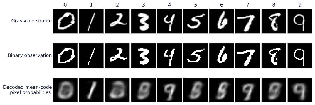
Data	12,000 training + 2,000 disjoint validation images from MNIST’s training split
Observation	Pixel/255 $>0.5$; all ten digit classes retained
Optimization	15 epochs, batch 256, Adam learning rate 0.001; 705 updates/model
Comparison	$\beta_{\mathrm{VAE}}\in\{0.1,1,4\}$; common initialization, batch order and noise streams
Validation	Same images and four common code draws/image; report NLL and KL separately

These are measured outputs of one controlled, finite-budget pilot.

CPU, one initialization seed; official test set unused. Labels only select a fixed gallery and color the latent map. This is not a convergence, robustness, or Colab-runtime claim. Full settings and metrics: pilot record. Practice menu.

Sum coordinates, then average images

reconstruction = F.binary_cross_entropy_with_logits(
    pixel_logits, x, reduction="none"
).sum(dim=1)                         # 784 pixel terms → (B,)
kl = 0.5 * (
    mu.square() + logvar.exp() - 1 - logvar
).sum(dim=1)                         # 2 latent terms → (B,)
loss = (reconstruction + beta_vae * kl).mean()  # images → scalar

$$\widehat L_\beta =\frac1B\sum_{i=1}^{B}\left[ -\ln p_\theta(x_i\mid u_i) +\beta_{\mathrm{VAE}}\operatorname{KL}(q_\psi(u\mid x_i)\Vert p(u))\right].$$

At $\beta_{\mathrm{VAE}}=1$, this estimates the negative ELBO.

One sampled code per image in training; exact latent KL. Separately averaging pixels and latent coordinates would change their relative weight. Gaussian sampling and reduction checks are reproducible in the pilot generator. Practice menu.

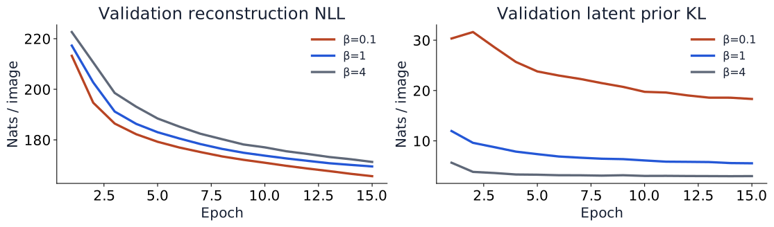
This pilot measured two competing pressures

In this run, larger $\beta$ reduced latent KL and increased reconstruction NLL.

Same validation examples and sampled noise, separate unweighted terms. Do not compare differently weighted total losses as a common quality metric. One seed and 705 updates per model; these observations are not a universal ordering. Original pilot. Practice menu.

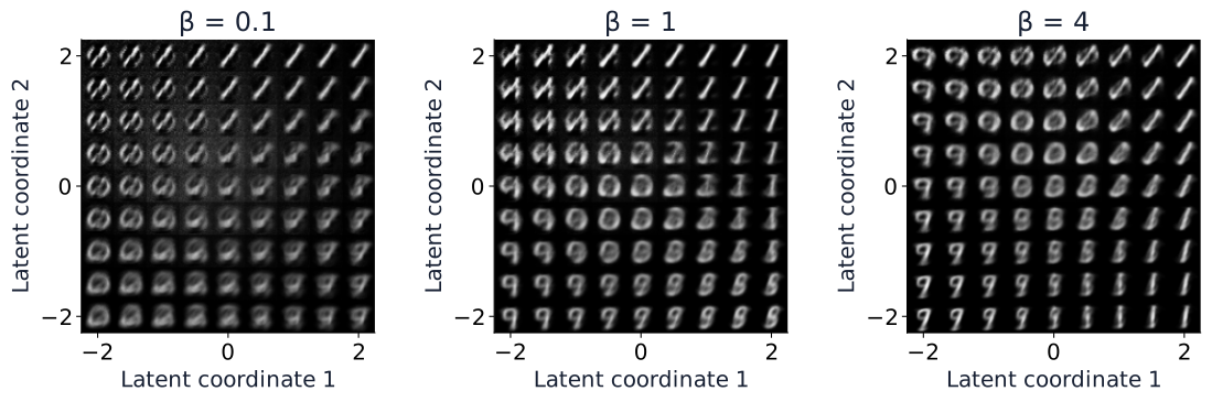
Compare the same latent region across models

Open discussion: compare recognizable and ambiguous regions. Expect differences in coverage; this grid alone cannot establish generation quality.

Chosen $9\times9$ coordinates in $[-2,2]^2$, not random prior samples. Every tile is a probability image. Inspect these alongside reconstruction NLL, latent KL, and actual prior draws; a grid alone does not establish generative quality. Practice menu.

Naive Bayes: two binary features

Toy classes $A,B$; stipulated model probabilities, not estimates from counts.

Class	Prior	$p(F_1=1\mid C)$	$p(F_2=1\mid C)$
$A$	0.4	0.8	0.7
$B$	0.6	0.2	0.3

Observe both features equal 1. Find $p(A\mid F_1=1,F_2=1)$. What permits the product?

Assume $F_1\perp F_2\mid C$: scores are $s_A=0.4(0.8)(0.7)=0.224$ and $s_B=0.036$. Normalize: $p(A\mid F_1,F_2)=0.224/0.260\approx0.862$.

Redundant features can count the same evidence twice and distort confidence. Count-based estimation needs an explicit smoothing choice for unseen combinations. Bishop, PRML §8.2. All practice · Return to Bayes.

Observation noise and parameter uncertainty

Method	What varies?	Prediction
Heteroscedastic head	Noise scale depends on input	Observation distribution at fitted weights
Bayesian regression	Weights have a posterior	Average over weights and observation noise
MC dropout	Stochastic network masks	Approximate predictive draws under assumptions

For a specified posterior predictive model: $$\operatorname{Var}(y_*\mid x_*,\mathcal D)= \mathbb E_\theta[\operatorname{Var}(y_*\mid x_*,\theta)] +\operatorname{Var}_\theta[\mathbb E(y_*\mid x_*,\theta)].$$ Observation spread and uncertainty in the predicted mean can coexist.

Dropout is not automatically calibrated Bayesian inference; its interpretation depends on modeling assumptions. Gal & Ghahramani (2016). All practice · Return to prediction.

Optional practice and worked answers

• RNN ledger and replay
• Counts, Steve and independence
• CDF, moments and general rules
• Heteroscedastic loss derivation
• Naive Bayes
• Inference frameworks
• Optional entropy/CE decomposition
• Noise versus weight uncertainty

• Beta update
• Prior strength
• Future-count prediction
• ELBO algebra and exact numbers
• Gaussian KL
• VAE implementation and pilot

Choose a task, reveal its answer, and return to the corresponding teaching frame.

Public, ungraded practice. Return to the lecture map · Tutorials. The main teaching route ends at the references.