Week 07 — From uncertain predictions to generating images
A fitted line makes one prediction. What other lines could explain the same measurements? Later, an encoder will give an image several plausible hidden codes. We will inspect both kinds of uncertainty, then use a decoder to generate new images.
Educational draft for instructor review. This is a guided reading with working code: predict what will happen, run a short calculation, and explain the resulting figure. The exercises ask you to change settings; no missing code blocks prevent Run all.
Route
Question
Suggested discussion time
1–2 · Regression
Which lines remain plausible after observing data?
20 min
3 · Dropout
What happens when prediction includes random masks?
10 min
4–6 · VAE anatomy
How does an image become a distribution of codes?
30 min
7–8 · Train and explore
Can we reconstruct, interpolate, and generate?
25 min
Interpretation
What was uncertain in each model?
5 min
Scene 2 derives the weight posterior from Bayes’ theorem. Scene 6 includes a 5–10 minute theory walkthrough connecting latent inference to the ELBO and the implemented loss. Both explanations are self-contained; the slides are optional companions.
Optional: a short Naive Bayes exercise. For a shorter class, skip the dropout comparison and optional exercises; keep the VAE walkthrough.
Learning objectives: distinguish parameter uncertainty from observation noise; read an encoder with two output heads; connect a regression posterior to Bayes’ theorem; explain reparameterization; derive the ELBO and its two VAE loss terms; distinguish reconstruction from generation.
Read and run:Open in Colab, or download and upload this notebook. Run cells in order. Use Python 3 with NumPy, Matplotlib, PyTorch, Torchvision, and IPython. No new library is needed beyond the existing course environment. The default path trains on a small thresholded MNIST subset on CPU; allow up to a few minutes of computation, depending on hardware, in addition to reading. A timer reports the actual run. MNIST is loaded from cache or downloaded in the explicitly labeled data cell. The offline check uses labeled synthetic patterns instead of digits.
TODO(instructor): review the educational text, 90-minute pacing, MNIST download/environment choice, and classroom subset size before release.
Notation: what is uncertain?
Symbol / code name
Meaning and shape
\(\mathcal D\), x_train, y_train
Observed training data; regression arrays of length \(n\)
\(\theta=(b,w)\)
Regression intercept and slope; column vector with 2 entries
\(X\), design
Regression design matrix \((n,2)\); each row is \([1,x_i]\)
\(\sigma^2\), NOISE_SD**2
Known observation-noise variance in the synthetic regression model
\(\tau^2\), PRIOR_SD**2
Variance of each independent zero-mean regression weight prior
Minimized loss and maximized evidence lower bound (ELBO)
The context distinguishes regression weights from decoder weights, both denoted \(\theta\) in the lecture. We retain \(u\) for latent codes, \(\psi\) for encoder weights, and \(\phi\) for activations; some papers instead use \(z\) and \(\phi\) for the first two.
Natural logarithms give losses in nats. For images, sum pixel contributions and latent-coordinate contributions within each image, then average across images. * on same-shaped tensors multiplies coordinatewise; @ is matrix multiplication. Batch rows contain observations; network features occupy columns.
Setup: imports and reproducible CPU settings
# @title Setup — run onceimport copyimport osimport timefrom pathlib import Pathimport numpy as npimport matplotlib.pyplot as pltimport torchfrom torch import nnfrom torch.nn import functional as Ffrom IPython.display import display, Markdownstarted = time.perf_counter()SEED =17EXPORT_FIGURES =False# Instructor setting; requires a local repository checkout.repository_root = Path.cwd().resolve()ifnot (repository_root /"_quarto.yml").exists(): repository_root = repository_root.parentfigure_directory = repository_root /"assets"/"figures"/"shared"/"week07"if EXPORT_FIGURES:assert (repository_root /"_quarto.yml").exists(), "Export from the repository or tutorials directory." figure_directory.mkdir(parents=True, exist_ok=True)plt.rcParams["svg.hashsalt"] ="week07-tutorial"np.random.seed(SEED)torch.manual_seed(SEED)torch.set_num_threads(2)plt.rcParams.update({"font.size": 11, "figure.dpi": 110})print(f"PyTorch {torch.__version__}; calculations and training use CPU.")
PyTorch 2.8.0; calculations and training use CPU.
Auxiliary figures
Run this folded cell once, then continue to Scene 1. Plotting and display functions live here so the scenes keep their calculations visible. Model definitions, posterior calculations, sampling, losses, and training remain beside their explanations. Figures are generated from this run; captions explain the same information in words.
Auxiliary plotting helpers (expand to edit the figures)
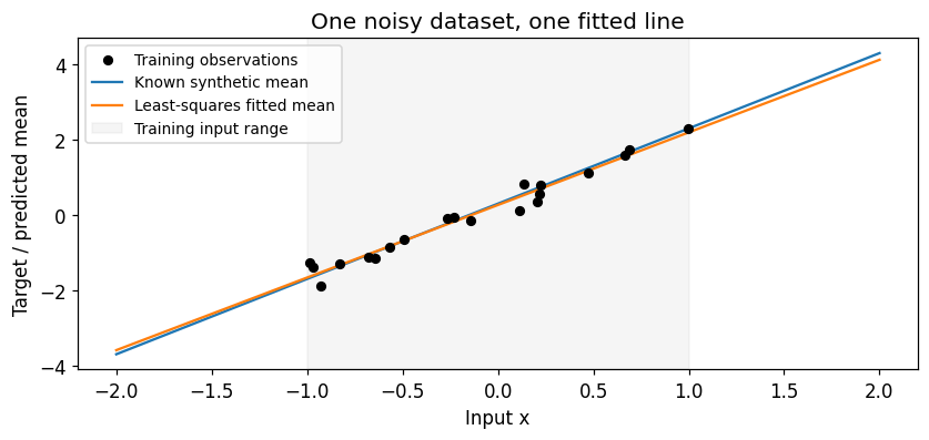
We know the generator because we wrote it. A learner sees only the observations. Here noise is independent across observations and has the same known standard deviation everywhere.
Draw three independent sets before fitting. Training fits the models; validation provides a descriptive check. The test set is reserved and remains unused throughout this tutorial. Inputs in all three sets lie in \([-1,1]\). The wider plotting grid is an extrapolation probe, not a test dataset.
The fitted line minimizes summed squared residuals. Under our common-variance Gaussian observation model, it also maximizes the likelihood. It gives a point estimate of \(\theta\); additional procedures would be needed to report uncertainty.
Pause: with only eight measurements, would you trust the fitted slope as much as with eighty? The next scene keeps several possible slopes and intercepts instead of selecting just one.
Scene 2 — Keep a distribution over lines
Why are the weights variables?
Our prediction rule is \(f_\theta(x)=b+wx\), with \(\theta=(b,w)^\top\). In the synthetic sensor model there is one fixed, unknown intercept and slope. The sensor does not draw new weights every time we measure it; repeated readings vary because of observation noise.
What varies in Bayesian inference is our uncertainty about the unknown weights. Before seeing enough data, several pairs \((b,w)\) could be plausible. A probability distribution over \(\theta\) describes that uncertainty. Drawing weights from it lets us inspect alternative explanations of the same observations. These draws are not gradient-descent updates.
Keep two operations separate. A point-estimation method changes candidate weights while searching for one fit. Bayesian inference updates a distribution over candidate weights when data arrive. The distribution can then supply a point summary, such as its mean, while retaining the spread around it.
1 · Put the regression model into Bayes’ theorem
Let \(y=(y_1,\ldots,y_n)^\top\) and let \(X\) be the design matrix with rows \([1,x_i]\). We condition on these observed inputs. Bayes’ theorem gives
The prior says which weights are plausible before these observations. The likelihood asks how well a particular candidate pair of weights explains the observed targets. The posterior combines them. The evidence normalizes the result:
Here \(v\) is a dummy variable ranging over possible weight pairs. The evidence depends on the data and the assumed model, but not on the candidate \(\theta\) in the numerator. To find the posterior’s shape, we can first write \(p(\theta\mid\mathcal D)\propto p(y\mid X,\theta)p(\theta)\), where \(\propto\) means “proportional to,” then normalize.
2 · Specify the prior and likelihood
Choose independent zero-mean Gaussian priors for intercept and slope:
The prior prefers values near zero, with strength controlled by PRIOR_SD\(=\tau\). It does not assert that the true slope is zero. Its scale depends on the chosen units. The noise scale \(\sigma\) and prior scale \(\tau\) are held fixed in this example.
This is a probability density over possible targets when \(\theta\) is fixed. After observing \(y\), we evaluate it as a function of candidate weights: the likelihood. The likelihood alone is not a normalized probability density over weights.
3 · Multiply the two factors and collect the quadratic terms
The remaining exponent is \(-\tfrac12[\theta^\top A\theta-2\theta^\top X^\top y/\sigma^2]\). Notice the two contributions to \(A\): prior information and information supplied by the observed inputs.
4 · Recognize the Gaussian by completing the square
Choose \(m\) so that \(Am=X^\top y/\sigma^2\). Then
\(S\) is the posterior covariance: its diagonal entries are the variances of intercept and slope; its off-diagonal entries describe their posterior covariance. \(A=S^{-1}\) is called precision. In this Gaussian model, prior precision and data precision add. A larger precision corresponds to a more constrained distribution.
This exact Gaussian answer relies on a linear mean \(X\theta\), fixed Gaussian noise, and a Gaussian weight prior. Gaussian observation noise plus a Gaussian weight prior does not generally give a Gaussian posterior for a nonlinear neural network.
5 · Match the equations to the next cell
posterior_precision implements \(A\). Solving \(AS=I_2\) gives the covariance. Solving \(Am=X^\top y/\sigma^2\) gives the mean, without explicitly constructing an inverse for that calculation. We keep both \(m\) and \(S\), then use them to draw plausible lines.
For this Gaussian posterior, its mean also equals its mode, so \(m\) is the MAP (maximum a posteriori) weight estimate. Keeping only \(m\) would lose the uncertainty stored in \(S\).
Checkpoint: what is observed and fixed when we evaluate the likelihood? What variable does the posterior describe? Why can the evidence be omitted while collecting terms in \(\theta\)?
PRIOR_SD =1.5# TODO(student): try 0.2 and 3.0, especially with little data.assert PRIOR_SD >0prior_precision = np.eye(2) / PRIOR_SD**2posterior_precision = prior_precision + design.T @ design / NOISE_SD**2posterior_cov = np.linalg.solve(posterior_precision, np.eye(2))posterior_mean = np.linalg.solve(posterior_precision, design.T @ y_train / NOISE_SD**2)assert np.all(np.linalg.eigvalsh(posterior_cov) >0)np.testing.assert_allclose(posterior_precision @ posterior_cov, np.eye(2), atol=1e-12)print("Posterior mean [intercept, slope]:", posterior_mean.round(3))print("Posterior standard deviations:", np.sqrt(np.diag(posterior_cov)).round(3))
Posterior mean [intercept, slope]: [0.264 1.921]
Posterior standard deviations: [0.058 0.095]
From uncertain weights to uncertain predictions
At a new input, let \(a_*=[1,x_*]\). The mean function is \(f_*=a_*\theta\). Its posterior variance is \(a_*Sa_*^\top\). A new noisy observation has an additional \(\sigma^2\):
\[\mathbb E[y_*\mid x_*,\mathcal D]=a_*m,\qquad
\operatorname{Var}(y_*\mid x_*,\mathcal D)=
\underbrace{a_*Sa_*^\top}_{\text{uncertainty in the mean}}+
\underbrace{\sigma^2}_{\text{observation noise}}.\]
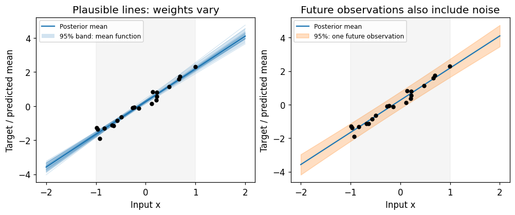
Draw plausible weights, then turn each draw into a whole line. One weight draw is shared across all inputs on that line. The two shaded bands below are pointwise intervals under this specified model; they are not simultaneous bands for the entire curve.
Validation RMSE (descriptive, no tuning):
  Least squares: 0.262
  Bayesian posterior mean: 0.263
Read the figure: the left panel varies the fitted mean because weights remain uncertain. The right panel includes new measurement noise. The mean-function band can become narrow with enough data; individual readings still scatter. Outside the observed input range, these straight-line predictions rely on the assumed linear relationship continuing to hold.
TODO(student): predict, then change N_TRAIN from 20 to 80 and rerun Scenes 1–2. What happens to the two bands? Next return to 20 and increase NOISE_SD to 0.6. Finally try a narrow prior. Describe separately the movement of the mean and the change in spread. Rerun the whole notebook when changing a setting used by later scenes.
# Verification: posterior draws reproduce the analytic mean-function variance.check_rng = np.random.default_rng(SEED +2)check_draws = check_rng.multivariate_normal(posterior_mean, posterior_cov, size=30000)probe = np.array([1.0, 0.5])np.testing.assert_allclose(np.var(check_draws @ probe), probe @ posterior_cov @ probe, rtol=0.04)# With the same noise model/prior, adding data cannot increase covariance.extra_design = np.column_stack([np.ones(120), x_pool])more_cov = np.linalg.solve(prior_precision + extra_design.T @ extra_design / NOISE_SD**2, np.eye(2))assert np.linalg.eigvalsh(posterior_cov - more_cov).min() >-1e-12print("Posterior covariance and sampling checks passed.")
Posterior covariance and sampling checks passed.
Scene 3 — A network with random masks
A tiny MLP gives us a familiar architecture with one new operation:
scalar input → 32 features → dropout → 32 features → dropout → scalar output
During training, dropout randomly zeros some hidden features and rescales the retained ones. At prediction time, ordinary eval() disables it. We will deliberately turn only the dropout layers back on and run several forward passes.
This is a short illustration of Monte Carlo (MC) dropout. Its Bayesian interpretation depends on modeling assumptions; repeated masks do not automatically provide calibrated uncertainty. Read Gal & Ghahramani (2016) for the approximate inference argument.
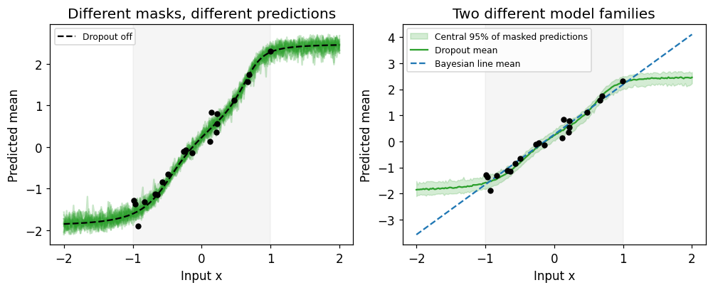
The Bayesian model is constrained to straight lines; the MLP can bend. Their different shapes and uncertainty mechanisms make this an exploration, rather than a ranking of inference methods.
DROPOUT_P =0.1# TODO(student): try 0.05 or 0.3; retrain after changing this.assert0<= DROPOUT_P <1torch.manual_seed(SEED)dropout_model = nn.Sequential( nn.Linear(1, 32), nn.Tanh(), nn.Dropout(DROPOUT_P), nn.Linear(32, 32), nn.Tanh(), nn.Dropout(DROPOUT_P), nn.Linear(32, 1),)x_tensor = torch.tensor(x_train[:, None], dtype=torch.float32)y_tensor = torch.tensor(y_train[:, None], dtype=torch.float32)grid_tensor = torch.tensor(grid[:, None], dtype=torch.float32)dropout_optimizer = torch.optim.Adam(dropout_model.parameters(), lr=0.01)# Full-batch training keeps this small example easy to read.dropout_model.train()for step inrange(500): dropout_optimizer.zero_grad() prediction = dropout_model(x_tensor) dropout_loss = F.mse_loss(prediction, y_tensor) dropout_loss.backward() dropout_optimizer.step()assert torch.isfinite(dropout_loss)print(f"Final masked training MSE: {dropout_loss.item():.4f}")
Final masked training MSE: 0.0377
Predict repeatedly with dropout active
First get the ordinary deterministic prediction. Then activate the dropout modules and collect 100 stochastic passes. Gradients are unnecessary for prediction. This model has no batch-normalization layers; selectively enabling dropout also avoids accidentally changing such layers in a larger model.
Read the figure: the green envelope summarizes sampled network outputs. We did not add observation noise to these draws, so it describes spread in the network’s mean predictions. It has a different meaning from the orange future-observation interval in Scene 2. Ordinary dropout also samples masks per batch entry; each displayed pass is a set of stochastic evaluations, not necessarily one coherent posterior function draw.
TODO(student): set DROPOUT_P = 0, rerun Scene 3, and explain what disappears. Then try 0.3 with fresh training. Does a wider envelope guarantee more accurate predictions? Compare inside and outside the training range without claiming calibration from one plot.
Transition: so far uncertainty affected a prediction. Now we will use a distribution inside an image architecture. The VAE’s distribution describes hidden codes for an image; the network weights themselves will be fitted point estimates.
Scene 4 — An image becomes a distribution
A deterministic autoencoder compresses an image to one code and decodes it. A variational autoencoder (VAE) adds a probabilistic structure: a prior for generating codes, a decoder distribution for images, and an encoder that approximates inference about codes.
For this tutorial, the latent prior is \(p(u)=\mathcal N(0,I_2)\). The encoder predicts an approximate posterior
There are two latent coordinates, each with its own mean and variance. The diagonal covariance assumes they are independent within this Gaussian approximation for one image. It does not imply that encoder means across different images are independent.
Network weights are learned point estimates. The encoder’s distribution is about an image’s hidden code, unlike Scene 2’s posterior over regression weights. We can write Bayes’ theorem for that code just as we wrote it for regression weights. A nonlinear decoder makes exact inference harder, so the encoder supplies an approximation. Scene 6 derives the training objective from that Bayes rule in a continuous, step-by-step walkthrough. The inference architecture and training principle follow Kingma & Welling, Auto-Encoding Variational Bayes.
architecture_figure()
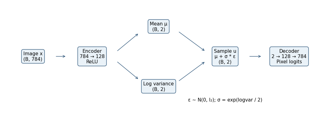
Architecture caption: a batch of 784-pixel images enters one shared encoder. Two heads output mean and log variance, both with shape (B, 2). Independent standard-normal noise is shifted and scaled to obtain a code; the decoder returns 784 pixel logits per image.
Load a small, clearly defined dataset
Use MNIST’s training split only. Choose disjoint training and validation indices before processing; the official test split remains untouched. Labels are kept for coloring a later plot and never enter the VAE loss.
We threshold each grayscale image at pixel / 255 > 0.5. The resulting binary observations match the decoder’s Bernoulli pixel model. Reconstruction displays will be grayscale probabilities, even though the targets are binary.
The settings below explicitly enable a one-time MNIST download if the cache is missing (about 12 MB compressed). Set DOWNLOAD_MNIST = False to require a cache. CI must use the offline pattern mode; it never downloads MNIST. In Colab, the cache usually needs populating once per runtime. Dataset background: the Torchvision MNIST documentation.
Thresholded MNIST: 8000 training / 1000 validation images.
The encoder has two heads
Flattening preserves 784 pixel values but discards the explicit 2D arrangement. Our small MLP is chosen for readable code; a convolutional VAE would add image-specific structure.
First create 128 learned features with a linear layer and ReLU. Two separate linear heads read the same features: one predicts the latent mean; the other predicts log variance. The variance is positive after exponentiation, so the log-variance head can output any real number.
The following modules will become parts of our final VAE. We reuse these exact objects when assembling it.
First image's mean: [-0.1   -0.084]
First image's standard deviations: [1.028 0.974]
These are outputs of an untrained encoder. They show shapes and operations, not meaningful learned image representations yet.
Pause: why does one image need four output numbers for a two-dimensional code? Two specify the center; two specify the spread. A code sample itself still contains only two numbers.
Scene 5 — Sample without breaking the gradient path
We would like to draw from the encoder’s Gaussian and still train the encoder using reconstruction error. Separate parameter-independent randomness from its transformation:
This is reparameterization. epsilon supplies fresh noise; mu and std tell us how to move and stretch it. The factor one half converts log variance to log standard deviation.
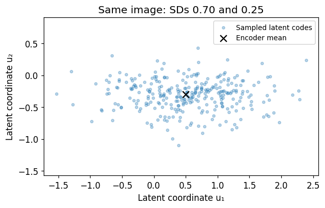
Begin with chosen numbers, independently of the untrained encoder. Fix the same noise samples while changing the settings below.
MU_DEMO = [0.5, -0.3] # TODO(student): change only the center first.STD_DEMO = [0.7, 0.25] # Then change one spread; both must be positive.mu_demo = torch.tensor(MU_DEMO, dtype=torch.float32, requires_grad=True)assertmin(STD_DEMO) >0logvar_demo = (2* torch.log(torch.tensor(STD_DEMO))).requires_grad_()epsilon_demo = torch.randn(300, 2, generator=torch.Generator().manual_seed(SEED))codes_demo = mu_demo + torch.exp(0.5* logvar_demo) * epsilon_demosampling_figure(mu_demo.detach().numpy(), np.array(STD_DEMO), codes_demo.detach().numpy())# One sampled coordinate: both center and spread have a differentiable path.mu_gradient, logvar_gradient = torch.autograd.grad(codes_demo[0, 0], (mu_demo, logvar_demo))expected_logvar_gradient =0.5* STD_DEMO[0] * epsilon_demo[0, 0]torch.testing.assert_close(mu_gradient, torch.tensor([1.0, 0.0]))torch.testing.assert_close(logvar_gradient[0], expected_logvar_gradient)print(f"First ε: {epsilon_demo[0].numpy().round(3)}")print(f"First u: {codes_demo[0].detach().numpy().round(3)}")print(f"du₁/dμ₁ = {mu_gradient[0]:.3f}; du₁/dlogvar₁ = {logvar_gradient[0]:.3f}")
First ε: [-1.046  1.231]
First u: [-0.232  0.008]
du₁/dμ₁ = 1.000; du₁/dlogvar₁ = -0.366
Sampling caption: changing MU_DEMO moves the sample cloud; changing STD_DEMO stretches it along a coordinate. The plotted cloud uses the same noise in each rerun.
During one backward pass, the sampled noise is held fixed. Gradients pass through the addition, multiplication, and exponential to both encoder heads. Later forward passes draw fresh noise. We fixed the noise here only to make the comparison visible.
Decode one sampled code
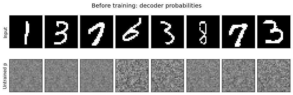
Now return to our actual image batch. The decoder produces logits, which the sigmoid maps to probabilities of white pixels. Given a code, we model pixel observations as conditionally independent Bernoulli draws. The shared code can still induce dependence between pixels when it is marginalized out.
The untrained outputs are close to gray because many probabilities are near one half. They are not successful reconstructions. We will reuse the same encoder and decoder in a trainable VAE.
Assemble the route
The class below registers the modules we already created and packages the operations we just inspected. Each method has one job. forward returns the quantities needed by the loss; decode returns logits so training can use a numerically stable loss.
class VAE(nn.Module):def__init__(self, encoder, mu_head, logvar_head, decoder):super().__init__()self.encoder = encoderself.mu_head = mu_headself.logvar_head = logvar_headself.decoder = decoderdef encode(self, x): features =self.encoder(x) # (B, 784) → (B, 128)returnself.mu_head(features), self.logvar_head(features)def reparameterize(self, mu, logvar, epsilon=None): std = torch.exp(0.5* logvar) # log variance → standard deviationif epsilon isNone: epsilon = torch.randn_like(std) # Fresh parameter-independent noisereturn mu + std * epsilon # Differentiable sampled codedef decode(self, u):returnself.decoder(u) # Pixel logits, not sampled pixelsdef forward(self, x, epsilon=None): mu, logvar =self.encode(x) u =self.reparameterize(mu, logvar, epsilon)returnself.decode(u), mu, logvarvae = VAE(encoder, mu_head, logvar_head, decoder)initial_vae_state = copy.deepcopy(vae.state_dict())# Same modules + same noise must reproduce the earlier explicit calculation.replayed_logits, replayed_mu, replayed_logvar = vae(batch_images, epsilon)torch.testing.assert_close(replayed_logits, pixel_logits)torch.testing.assert_close(replayed_mu, mu)torch.testing.assert_close(replayed_logvar, logvar)print(f"Registered trainable parameters: {sum(p.numel() for p in vae.parameters()):,}")
Registered trainable parameters: 202,516
Scene 6 — Two terms train the VAE
From Bayes’ theorem to the ELBO: a 5–10 minute walkthrough
We have seen what the encoder and decoder compute. Now follow one question: how can we train these networks when the exact posterior over an image’s code is difficult to calculate? Read the following steps in order; each equation answers the question left by the previous one.
1 · Specify a generator before asking it to infer anything
For one image, the generative story is: draw a hidden code \(u\) from \(p(u)=\mathcal N(0,I_2)\), then draw pixels from the decoder distribution \(p_\theta(x\mid u)\). The product rule gives the joint distribution
\[p_\theta(x,u)=p(u)p_\theta(x\mid u).\]
The decoder weights \(\theta\) are shared across all images. Each image has its own unobserved code \(u\). Our VAE learns one set of decoder weights; it does not maintain a Bayesian posterior over those weights.
This is the connection to regression: the same Bayes rule applies, but the unknown we infer is different.
Earlier regression
This VAE, for a fixed decoder
Observations: targets \(y\) at inputs \(X\)
Observation: image \(x\)
Unknown: shared weights \(\theta\)
Unknown: the image’s code \(u\)
Prior: \(p(\theta)\)
Prior: \(p(u)\)
Likelihood: \(p(y\mid X,\theta)\)
Likelihood: \(p_\theta(x\mid u)\)
Posterior: \(p(\theta\mid\mathcal D)\)
Posterior: \(p_\theta(u\mid x)\)
2 · State what learning a good generator would mean
We observe images, not their generating codes. To score an observed image, average over all possible codes under the prior:
\[p_\theta(x)=\int p_\theta(x\mid u)p(u)\,du.\]
This is the evidence, also called the marginal likelihood. It measures how much probability the whole generative model assigns to the image, after accounting for all possible hidden explanations. It is not the likelihood at one chosen code.
For independent training images, a natural learning objective would be to maximize
\[\sum_i\log p_\theta(x_i).\]
However, a nonlinear neural decoder generally makes the evidence integral impractical to evaluate exactly. Even two latent coordinates do not guarantee a simple analytic integral.
This posterior answers: which codes could plausibly have produced this particular image? At a chosen code we can evaluate the prior and decoder likelihood. The difficult denominator is exactly the evidence integral from Step 2.
So two tasks share one obstacle: we want to learn from image evidence, and we want to infer hidden codes, but we cannot conveniently calculate the exact evidence or posterior.
4 · Introduce an encoder as an approximate inference model
Choose a tractable distribution \(q_\psi(u\mid x)\) and let the encoder predict its parameters. In our code, this is the diagonal Gaussian specified by mu and logvar. A Gaussian prior does not make the nonlinear decoder’s exact posterior Gaussian. Our chosen family can miss correlated codes or several separated groups of plausible codes.
The encoder’s output is a proposal for the posterior, not an application of Bayes’ rule that magically computes the exact answer. “Variational” means that we vary a chosen family of approximating distributions to make the approximation useful. The shared encoder weights \(\psi\) let one network perform this inference for many images, instead of optimizing a separate inference procedure from scratch for every image.
We still need a way to train \(q\) without supplying exact posterior targets. That is the purpose of the next three steps.
5 · Use Bayes’ theorem to separate evidence from the inference gap
For this derivation, fix \(x\) and \(\theta\) and abbreviate \(q_\psi(u\mid x)\) as \(q(u)\). The expectation \(\mathbb E_q\) averages over possible codes drawn from this distribution.
KL divergence measures the discrepancy from \(q\) to the exact posterior:
Why did \(\log p_\theta(x)\) leave the expectation? The observed image and decoder are fixed here, so that quantity is constant as \(u\) varies. An average of a constant is the same constant.
Name the remaining expectation the evidence lower bound, or ELBO:
KL is nonnegative, so \(\mathcal E\le\log p_\theta(x)\). The gap is zero if \(q\) equals the exact posterior. For a fixed decoder, maximizing the ELBO is therefore equivalent to minimizing this inference gap. We assume positive evidence and finite expectations with suitable support.
The gap explains the mathematics; it is not a term we calculate against an unavailable exact posterior during training.
6 · Rewrite the bound into two computable terms
Expand the joint from Step 1 inside the ELBO:
\[\begin{aligned}
\mathcal E
&=\mathbb E_q[\log p_\theta(x\mid u)+\log p(u)-\log q(u)]\\
&=\underbrace{\mathbb E_q[\log p_\theta(x\mid u)]}_{\text{explain the observed pixels}}
-\underbrace{\operatorname{KL}(q_\psi(u\mid x)\Vert p(u))}_{\text{compare the encoder distribution with the prior}}.
\end{aligned}\]
The evidence integral has disappeared from this computable expression. We estimate the first term by sampling codes from \(q\). The second term has an analytic formula for our diagonal Gaussian and standard-normal prior.
There are two different KL divergences in the argument:
Comparison
Its job
Computed in our loss?
\(\operatorname{KL}(q\Vert p_\theta(u\mid x))\)
Gap between the bound and exact log evidence
No; the exact posterior is unavailable
\(\operatorname{KL}(q\Vert p(u))\)
Prior-comparison term inside the usable bound
Yes; analytic Gaussian formula
Matching the exact posterior makes the gap zero. It need not make the prior KL zero: seeing an image usually changes what we believe about its code.
7 · Turn a maximized bound into the minimized loss in Python
NLL means negative log likelihood. For each image, sample \(\epsilon\sim\mathcal N(0,I_2)\) and form \(u=\mu_u+\sigma_u\odot\epsilon\). With one sample, the stochastic loss estimate is
Average these estimates across the minibatch. The reconstruction gradient passes through the decoder, sampled code, and reparameterization to both encoder heads. The prior KL supplies additional encoder gradients. The optimizer updates both encoder weights \(\psi\) and decoder weights \(\theta\); it does not store the sampled \(u\) as a trainable parameter.
We maximize a bound while learning both networks. Because changing \(\theta\) also changes the evidence and exact posterior, an improvement in the joint ELBO does not by itself guarantee an improvement in exact evidence. Also, the bound applies to the expected ELBO; an individual Monte Carlo estimate need not lie below log evidence.
8 · Follow the argument into the code
Mathematical action
Notebook operation
Propose \(q_\psi(u\mid x)\)
encode(x) returns mu, logvar
Sample a plausible code from \(q\)
reparameterize(mu, logvar)
Specify \(p_\theta(x\mid u)\)
decode(u) returns pixel logits
Score the observed binary pixels
Sum binary_cross_entropy_with_logits over pixels
Compare \(q\) with \(p(u)\)
Sum the analytic Gaussian KL over coordinates
Minimize a minibatch negative-ELBO estimate
Add the terms, average images, backpropagate, update
There are no labels for the true latent codes and no exact posterior targets. The bound trains the encoder and generator together using the observed images. The standard VAE gives the prior KL coefficient one; changing that coefficient changes the objective.
Checkpoint: explain the route aloud: generative model → evidence → Bayes posterior → approximate encoder → ELBO identity → two computable terms → sampled training loss. Which integral was difficult? Which KL explains the gap? Which KL appears in the code?
Reference: Kingma & Welling, Auto-Encoding Variational Bayes, §2.2, equations (1)–(3), and §§2.3–2.4. Here the paper’s \(z,\phi\) become the course’s \(u,\psi\); we use \(\mathcal E\) for the maximized bound and \(L\) for the minimized loss.
Calculate the terms before combining them
Now implement Step 7 for the binary-image generator. Conditional independence of pixels given \(u\) makes their log likelihoods add. Use binary_cross_entropy_with_logits directly on logits. reduction="none" retains every pixel contribution; sum pixels for each image.
For the diagonal-Gaussian prior KL, sum the two coordinate contributions:
This is the prior KL from Step 6, not the unknown posterior gap. It is zero when every coordinate has mean zero and variance one. It penalizes departure from the prior in both center and spread, without demanding that every image’s approximate posterior equal the prior exactly.
Why does the reconstruction term initially look large? An uninformative probability of one half costs about ln(2) per binary pixel. With 784 pixels, those small costs add to roughly 543 nats per image.
We next put the same calculation in a reusable function. It returns per-image terms so the training loop can average them and the reports can keep them separate. The optional beta setting multiplies KL; the standard VAE uses beta = 1. Other values change the objective and should be labeled as such.
def vae_terms(logits, x, mu, logvar): reconstruction = F.binary_cross_entropy_with_logits(logits, x, reduction="none").sum(1) kl =0.5* (mu.square() + logvar.exp() -1- logvar).sum(1)return reconstruction, kl# Independent library check of the analytic KL formula.q = torch.distributions.Normal(mu, torch.exp(0.5* logvar))prior = torch.distributions.Normal(torch.zeros_like(mu), torch.ones_like(mu))library_kl = torch.distributions.kl_divergence(q, prior).sum(1)torch.testing.assert_close(kl_per_image, library_kl)zero = torch.zeros(3, 2)_, zero_kl = vae_terms(torch.zeros(3, 784), images_train[:3], zero, zero)torch.testing.assert_close(zero_kl, torch.zeros(3))# Trace one complete backward pass, without changing weights yet.vae.zero_grad()checked_logits, checked_mu, checked_logvar = vae(batch_images, epsilon)checked_nll, checked_kl = vae_terms(checked_logits, batch_images, checked_mu, checked_logvar)(checked_nll + checked_kl).mean().backward()for name, module in [("Encoder", vae.encoder), ("Mean head", vae.mu_head), ("Log-variance head", vae.logvar_head), ("Decoder", vae.decoder)]: gradients = [p.grad for p in module.parameters()]assertall(g isnotNoneand torch.isfinite(g).all() for g in gradients) norm =sum(g.square().sum().item() for g in gradients)**0.5assert norm >0print(f"{name} gradient norm: {norm:.3f}")vae.zero_grad()
Encoder gradient norm: 8.108
Mean head gradient norm: 3.434
Log-variance head gradient norm: 3.908
Decoder gradient norm: 46.786
Checkpoint: which dimension do we sum for pixels? Which for latent coordinates? Which dimension do we average? Changing a pixel sum to a pixel mean alone changes the relative influence of KL by a factor of 784.
At this point we have derived the objective from Bayes’ theorem and checked its operations, tensor shapes, Gaussian KL, and gradient flow through both heads. The next experiment uses that objective to train the image model.
Scene 7 — Train the model we just opened
Each minibatch follows the same familiar loop: predict, calculate loss, clear old gradients, backpropagate, update weights. Sampling happens inside forward on every batch.
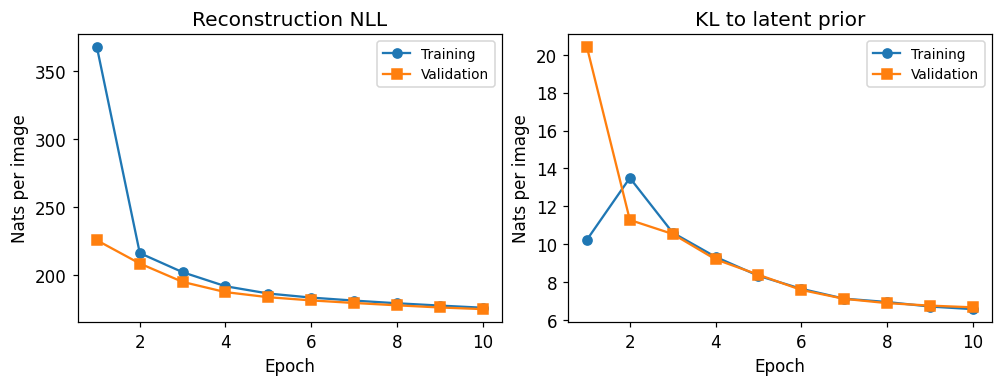
We use a fixed epoch budget rather than selecting an epoch after seeing results. Validation is held out from optimization. Its reconstruction NLL averages four fixed noise draws per image, so changes across epochs are easier to inspect. It is still a Monte Carlo estimate, not exact image evidence.
Measure validation without updating weights
The KL needs no sampling. We average sampled reconstruction terms over the four draws and accumulate sums across images. The final division reports nats per image, including a smaller final batch correctly.
The function below makes retraining explicit and reusable for the optional comparison. It owns its optimizer, shuffles training indices each epoch, and samples fresh latent noise. Resetting the two random streams makes the optional comparison use the same batch order and noise sequence.
The training report averages losses encountered while weights were changing during the epoch. Validation evaluates the weights at the end of that epoch. This difference can matter when comparing the two curves.
def train_vae(model, images, validation_images, epochs, beta, noise): optimizer = torch.optim.Adam(model.parameters(), lr=0.001) order_rng = torch.Generator().manual_seed(SEED +20) torch.manual_seed(SEED +21) # Latent noise; separate from batch ordering. history = []for epoch inrange(epochs): model.train() order = torch.randperm(len(images), generator=order_rng) total_nll, total_kl =0.0, 0.0for ids in order.split(256): x = images[ids] optimizer.zero_grad() logits, mu, logvar = model(x) reconstruction, kl = vae_terms(logits, x, mu, logvar) loss = (reconstruction + beta * kl).mean()assert torch.isfinite(loss), "Non-finite loss: inspect the settings." loss.backward() optimizer.step() total_nll += reconstruction.detach().sum().item() total_kl += kl.detach().sum().item() val_nll, val_kl = evaluate_vae(model, validation_images, noise) row = {"train_nll": total_nll/len(images), "train_kl": total_kl/len(images),"val_nll": val_nll, "val_kl": val_kl}assertall(np.isfinite(value) for value in row.values()) history.append(row)print(f"Epoch {epoch+1:2d}/{epochs}: "f"validation reconstruction {val_nll:.2f}, KL {val_kl:.2f} nats/image")return history
Run the standard VAE
Start from the exact modules inspected above. The assembly cell saved their initial weights for the optional paired experiment; rerunning the training cell restores those weights. Ten short epochs are a teaching budget; this is not a state-of-the-art digit generator.
TODO(student): after completing the default run, try five or fifteen epochs. Predict which outputs might improve. Keep the validation set fixed, and describe the observed change without treating repeated exploration as a final test.
EPOCHS =10BETA_VAE =1.0# Standard VAE; keep this at one for the main walkthrough.assertisinstance(EPOCHS, int) and EPOCHS >0assert BETA_VAE >0vae.load_state_dict(initial_vae_state) # Rerunning this cell starts fresh.before_nll, before_kl = evaluate_vae(vae, images_validation, validation_noise)training_started = time.perf_counter()history = train_vae(vae, images_train, images_validation, EPOCHS, BETA_VAE, validation_noise)training_seconds = time.perf_counter() - training_startedprint(f"Training took {training_seconds:.1f} seconds on this machine.")history_figure(history)last = history[-1]display(Markdown(f"**This run ({DATA_NAME}, beta={BETA_VAE:g}):** validation reconstruction NLL "f"changed from **{before_nll:.2f}** to **{last['val_nll']:.2f}** nats/image; "f"final prior KL is **{last['val_kl']:.2f}** nats/image. ""Read the two terms separately; they describe different pressures."))
This run (Thresholded MNIST, beta=1): validation reconstruction NLL changed from 551.80 to 175.18 nats/image; final prior KL is 6.67 nats/image. Read the two terms separately; they describe different pressures.
Training-curve caption: reconstruction NLL and prior KL are plotted in separate panels. Validation observations never supply optimizer gradients. These values describe this initialization, subset, and training budget; a single seed does not establish a general architecture ranking.
Scene 8 — Reconstruct, move, generate
Reconstruct an observed image
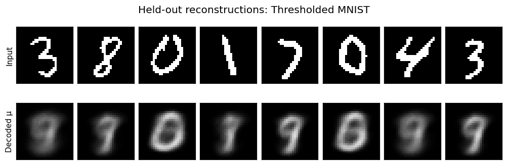
Encode validation images, then decode their mean codes. This deterministic display is convenient for comparison. It differs from the sampled reconstruction term used during training and validation scoring.
Reconstruction caption: the top row contains held-out binary inputs; the bottom row contains decoded pixel probabilities. A gray pixel means intermediate probability, not a third outcome in our binary observation model. A two-dimensional code and short training budget limit detail.
Look at the learned code space
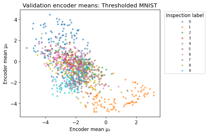
Place each validation image at its encoder mean. Color by labels for inspection only. The VAE was not trained to classify these labels, and two dimensions need not separate them cleanly. This scatter shows centers across images; it omits each image’s predicted spread.
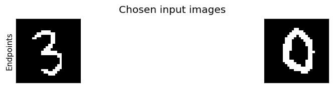
Choose two validation image indices. Interpolate linearly between their mean codes, then decode the path. This is a coordinate experiment; it is neither a prior sample nor proof that every intermediate image is realistic.
TODO(student): change the endpoint indices. Does the transition look smooth? Does smoothness guarantee a recognizable intermediate digit? Compare the endpoints with their reconstructions.
IMAGE_A =0IMAGE_B =5assert0<= IMAGE_A <len(images_validation) and0<= IMAGE_B <len(images_validation)alpha = torch.linspace(0, 1, 8)[:, None]code_a = validation_mu[IMAGE_A]code_b = validation_mu[IMAGE_B]interpolated_codes = (1-alpha)*code_a + alpha*code_bwith torch.no_grad(): interpolated_probabilities = torch.sigmoid(vae.decode(interpolated_codes))image_gallery([images_validation[[IMAGE_A, IMAGE_B]]], ["Endpoints"], "Chosen input images", n=2)image_gallery([interpolated_probabilities], ["Decoded"], "From mean code A (left) to mean code B (right)")
Generate from the prior
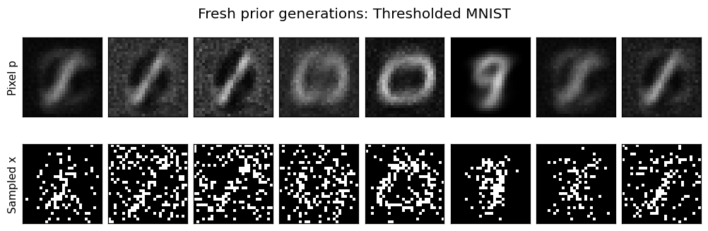
Reconstruction starts with an image. Generation starts with a fresh code from N(0, I₂) and uses only the decoder. Show both decoder probabilities and binary pixel samples. The latter are actual observations drawn from the Bernoulli image model. They can look speckled: every uncertain pixel is sampled independently given the code. Smooth probability images and sampled binary images answer different questions.
TODO(student): change GENERATION_SEED. Which outputs change? Why do we not call the encoder here?
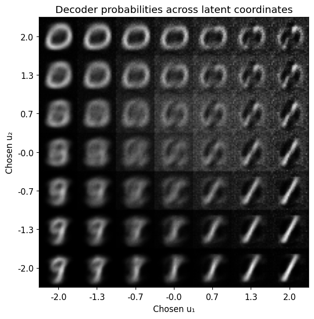
Decode a grid of chosen coordinates. Each tile is a probability image. This grid uses evenly spaced coordinates, while independent prior samples concentrate around the origin.
TODO(student): change GRID_LIMIT from 2 to 4. Describe what happens far from the origin. Those coordinates may be poorly supported by the prior and learned codes; the decoder still returns an output.
Complete the default walkthrough first. Then set RUN_BETA_EXPERIMENT = True and choose a second positive KL weight. Train a fresh copy from the saved initial weights with the same subset, epoch count, optimizer, batch order, and latent noise stream. The standard VAE above remains available for the main galleries.
Predict how reconstruction and KL might respond before running. Compare unweighted validation terms, rather than total losses with different coefficients. Stronger KL pressure does not guarantee monotonic results or better generated images under finite training.
Optional fresh paired training run (off by default)
# @title Optional: compare one different KL weightRUN_BETA_EXPERIMENT =FalseSECOND_BETA =4.0# TODO(student): try 0.1 or 4.0; write your prediction first.assert SECOND_BETA >0if RUN_BETA_EXPERIMENT: alternate_vae = copy.deepcopy(vae) alternate_vae.load_state_dict(initial_vae_state) alternate_history = train_vae(alternate_vae, images_train, images_validation, EPOCHS, SECOND_BETA, validation_noise) alternate_last = alternate_history[-1] display(Markdown("| KL weight | Reconstruction NLL | Prior KL |\n|---|---:|---:|\n"f"| {BETA_VAE:g} | {last['val_nll']:.2f} | {last['val_kl']:.2f} |\n"f"| {SECOND_BETA:g} | {alternate_last['val_nll']:.2f} | {alternate_last['val_kl']:.2f} |\n\n""All values are nats/image on the same validation observations and noise draws." ))with torch.no_grad(): alternate_prior_probabilities = torch.sigmoid(alternate_vae.decode(prior_codes)) image_gallery([generated_probabilities, alternate_prior_probabilities], [f"β={BETA_VAE:g}", f"β={SECOND_BETA:g}"], "Same prior codes, two trained decoders")else:print("Optional training is off. The main VAE experiment is complete.")
Optional training is off. The main VAE experiment is complete.
Optional exercise — Naive Bayes in a few lines
Return to the lecture’s two binary features. The stipulated model has classes \(A,B\), priors \((0.4,0.6)\), and feature probabilities shown in the code below. These are synthetic assumptions, not estimates from a real dataset.
Conditional independence lets us multiply feature likelihoods within each class:
This is Bayes’ rule for a class label, not necessarily Bayesian inference over uncertain classifier parameters. The table parameters here are fixed.
TODO(student): before running, predict the favored class for two present features. Change PRIOR_A, then change the observed features. Finally duplicate the first feature using DUPLICATE_FIRST = True; explain why treating repeated evidence as independent changes confidence without supplying new information.
Class scores [A, B]: [0.224 0.036]
Posterior class probabilities: [0.8615 0.1385]
What did we learn?
Complete three short statements using your own outputs:
Regression: after changing data count or noise, the mean-function band …, while the future-observation band …, because … .
Dropout, if run: repeated masks varied … . This figure alone does not establish … .
VAE: the encoder supplies …; reparameterization lets …; the decoder supplies … . Reconstruction starts with …, whereas generation starts with … .
The common idea is to specify what varies and which distribution describes it. Regression kept a posterior over weights. MC dropout varied network masks. The VAE learned an approximate distribution over each image’s latent code and a decoder distribution over binary pixels.
This tutorial used one reproducible initialization and small datasets. Validation supported exploration; both the regression test set and MNIST’s official test split remained unused. No result establishes universal superiority or calibrated uncertainty under distribution shift.
References:Week 07 lecture; Bishop, PRML §3.3 for Bayesian linear regression and §8.2 for graphical-model factorization; Gal & Ghahramani (2016) for dropout; Kingma & Welling §§2–3 and Appendix B for the VAE. Plots and diagrams are original course calculations; image galleries use MNIST via Torchvision, or explicitly labeled procedural patterns in offline checks. The trained outputs here come from this notebook, independently of the lecture’s longer pilot.
TODO(instructor): accept the teaching text, figures, experiment settings, and pacing before publication. The synthetic-rainfall decision in the earlier Week 07 draft is superseded by the instructor-approved regression/VAE scope; no real-weather claim is used here.
assert torch.isfinite(validation_mu).all()assert torch.isfinite(validation_logvar).all()assertlen(history) == EPOCHSprint(f"Completed: {DATA_NAME}; {N_IMAGES_TRAIN} training images, {EPOCHS} epochs, beta={BETA_VAE:g}.")print(f"Computation since setup: {time.perf_counter()-started:.1f} seconds (includes any interactive pauses).")
Completed: Thresholded MNIST; 8000 training images, 10 epochs, beta=1.
Computation since setup: 4.6 seconds (includes any interactive pauses).