← Course homeAll chapters

Week 06 · Sequential Representation Learning: From Recurrent Memory to Transformer Encoders

English · Русский

“A journey of a thousand miles begins…” invites a continuation. The next word depends on the words already supplied and on their arrangement. Measurements have a similar structure: a rising temperature and a falling temperature can have the same average, yet suggest different next measurements. A representation for a sequence must preserve the information that its task needs.

Week 04 explained how a model learns intermediate representations. Week 05 reused parameters across image locations. Here we reuse parameters across positions in a sequence, and ask how information can move between those positions. A recurrent model carries a state from one observation to the next. Attention constructs a representation by combining information from available source positions. Both still require a prediction head, a loss, and a learning procedure.

We will begin with one input number and one state number. That small model lets us see every operation in the forward pass and every link in the backward pass. Later sections will expand to vector states, examine memory gradients and gates, and build attention and a complete Transformer encoder around the seven-word prefix above.

Learning outcomes

After reading this chapter, you should be able to:

1. define a sequence task and the information available when a prediction is made;
2. compute recurrent states and predictions, and derive gradients from every use of shared parameters;
3. explain how sequence length, activation derivatives, and gated updates affect memory and learning;
4. trace tokens through embedding lookup, positional information, and single- and multi-head attention;
5. explain the operations, axes, residual paths, and task heads of a Transformer encoder; and
6. check masking, target alignment, and sequence evaluation, and interpret the evidence a comparison supports.

Prerequisites and companion materials

We assume scalar derivatives and the chain rule. The Week 04 chapter explains why derivatives multiply along a path and add where paths meet. The Week 05 chapter shows how one shared parameter receives contributions from several uses. Matrix multiplication will become useful when we expand to vector states; it is not needed for the first calculation.

The Week 06 lecture provides the teaching overview. The Week 06 tutorial makes sequence learning executable through a tiny robot-command language. This chapter’s scalar regression example is a separate, deliberately small calculation; it develops the formulas without assigning numerical values to the observations, weights, or target.

Why order and available context matter

State the prediction problem first

A sequence is an ordered collection of observations. Write its positions as \(t=0,\ldots,T-1\), where \(T\) is its length. An observation might be one sensor value, a vector of measurements, or a token identifying a word. We start with a scalar observation \(x_t\in\mathbb R\): one real number at each position.

The output need not have the same structure as the input. We might assign one class to a complete sequence, label every supplied word, or forecast a future measurement from an observed prefix. These tasks differ in what a prediction may use.

Table 1: Sequence tasks determine both the output and the information available for prediction.

Task	Prediction	Available input in the stated task
Classify a recorded sequence	One label for the recording	The complete supplied recording
Label words in a supplied sentence	One label per word	The complete sentence, if the application permits it
Forecast the next measurement	One future value	Measurements observed before that future value

A prefix consists of the observations supplied so far, in order. For forecasting, the unknown next observation is a target, not part of that prefix. A model receiving future measurements during training would answer an easier question than the one it must answer at deployment. We therefore specify the available input before choosing the architecture.

NotePause and predict: what may a forecast use?

You have observed \(x_0,x_1,x_2\) and must predict the next measurement \(x_3\). Which observations may enter the prediction? If a training example also contains the true \(x_3\), where does that value belong?

Reveal the explanation

The prediction may use the observed prefix \(x_0,x_1,x_2\). The true \(x_3\) supplies the target for the loss. Supplying it to the predictor would reveal the answer that is unavailable when a future measurement must be forecast.

Carry a representation through the sequence

For a fixed length, we can supply \((x_0,x_1,\ldots,x_{T-1})\) to a feedforward model. Each coordinate has a position, so flattening in a declared order does not erase order. A recurrent model offers a different construction: apply the same small transformation repeatedly, combining the current observation with the previous representation.

Its hidden state \(h_t\) is the representation after processing position \(t\). “Hidden” means intermediate: the state is inside the prediction computation, rather than an observed measurement or a target. In our scalar model, it is one real number summarizing the computation on the prefix. It need not reproduce the observations or preserve every detail of them.

Each step uses \(x_t\) and \(h_{t-1}\). The parameters stay the same while the state changes. A longer sequence adds more uses of that transformation; it does not require a separate set of cell parameters at every position. This is parameter sharing across time, analogous to Week 05’s sharing across spatial locations. The recurrent construction and its unrolled computation graph are described in Goodfellow et al. (2016), Chapter 10.

One scalar recurrent model: forward pass, prediction, loss, and learning

State the three-step problem

Suppose one training example contains three scalar observations, \((x_0,x_1,x_2)\), and one scalar target \(y\). Thus the sequence length is \(T=3\), and its time steps are \(t=0,1,2\). We will process these observations in order, then predict \(y\) from the final state. For forecasting, \(y\) could be the next measurement \(x_3\); the derivation only requires a supplied regression target.

A recurrent neural network (RNN) repeatedly applies a cell, the transformation that combines the current observation with the previous hidden state. For scalar input \(x_t\) and scalar state \(h_t\), write

\[ z_t=w_xx_t+w_hh_{t-1}, \qquad h_t=\phi(z_t). \]

The input weight \(w_x\) controls the contribution of the current observation, and the recurrent weight \(w_h\) controls the contribution of the previous state. The preactivation \(z_t\) is the value before applying the activation function \(\phi\); the hidden state \(h_t\) is the value afterward. We leave \(\phi\) general and assume it is differentiable at the preactivations in the example.

For this derivation, both the cell bias and the output bias are fixed at zero. They are omitted from the formulas and updates. The trainable parameters are the three weights \(\theta=(w_x,w_h,w_o)\). Biases can be restored in a more general model; leaving them out here lets us follow the recurrent dependencies directly.

Before the first observation, set the fixed initial state to \(h_{-1}=0\). This is a starting condition, not a fourth observation. Independent sequences start with a fresh initial state under this model.

A prediction head, also called a readout, turns a hidden state into a regression prediction. At a position where an output is needed, it applies

\[ \widehat y_t=w_oh_t. \]

Figure 1 shows both operations: the recurrent cell produces \(h_t\), and the output head reads it. The cell itself is the same at every time step: it reuses \(w_x,w_h\) and \(\phi\). Its state \(h_t\) changes with the observations. The prediction \(\widehat y_t\) is an output; it is \(h_t\) that feeds the next recurrent step. The diagram labels the current-input and previous-state contributions as \(I_t=w_xx_t\) and \(R_t=w_hh_{t-1}\).

Figure 1: The recurrent cell produces a hidden state for the next time step; a separate output head can read that state through w_o. This example reads only the final state. Biases are fixed at zero. Original course diagram.

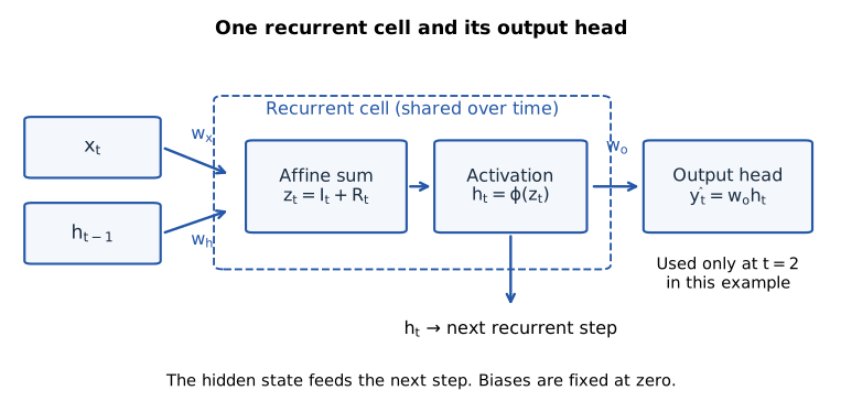
Our three-step problem requires one prediction after the final time step, so we apply the head only to \(h_2\) and write \(\widehat y=\widehat y_2\). The loss is

\[ \widehat y=w_oh_2, \qquad \mathcal L=\frac12(\widehat y-y)^2. \]

The output weight \(w_o\) converts the hidden representation into the prediction \(\widehat y\). The target \(y\) determines the prediction error and the loss \(\mathcal L\). There is one final-output loss; no loss is attached to an earlier time step. The factor \(1/2\) simplifies differentiation. There is no averaging over positions or examples here. This \(\mathcal L\) is a particular instance of Week 04’s generic loss \(L\).

Table 2: Symbols for the three-step scalar model and its backward sensitivities. The superscripts on \(g_t^h\) and \(g_t^z\) are labels, not powers.

Symbol	Meaning in this example
\(x_0,x_1,x_2\)	Three observed scalar inputs
\(h_{-1}=0\)	Fixed initial state
\(z_t\), \(h_t\)	Preactivation and hidden state at time step \(t\)
\(w_x\), \(w_h\)	Input and recurrent weights, shared over time
\(w_o\)	Weight of the output head; used only at the final step in this example
\(\phi\), \(\phi'\)	Activation and its local derivative
\(y\), \(\widehat y\), \(\mathcal L\)	Target, final prediction, and one-sequence loss
\(\widehat y_t=w_oh_t\)	A prediction read from state \(h_t\) when the task needs an output at position \(t\)
\(e=\widehat y-y\)	Prediction error; also \(\partial\mathcal L/\partial\widehat y\) for this squared-error loss
\(g_t^h=\partial\mathcal L/\partial h_t\)	Loss sensitivity to the hidden state at time step \(t\); superscript \(h\) labels the differentiated variable
\(g_t^z=\partial\mathcal L/\partial z_t\)	Loss sensitivity to the preactivation at time step \(t\); superscript \(z\) labels the differentiated variable

Match each forward operation to its backward calculation

Unrolling draws each use of the same recurrent cell separately. In Figure 2, the final loss depends on \(h_2\), which depends on \(h_1\), which depends on \(h_0\). Each box uses the same \(w_x,w_h\); increasing the number of boxes does not introduce independent weights.

Figure 2: Three time steps produce a final hidden state, a prediction, and a loss. Backpropagation follows the recorded dependencies in reverse using the same weights. Original course diagram.

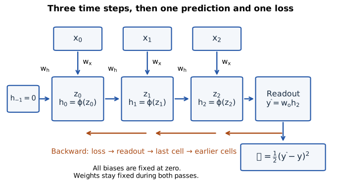
For any scalar intermediate value \(v\), \(\partial\mathcal L/\partial v\) describes how a small change in \(v\) would affect the loss through the remaining computation. We will use short names for two such sensitivities:

\[ g_t^h=\frac{\partial\mathcal L}{\partial h_t}, \qquad g_t^z=\frac{\partial\mathcal L}{\partial z_t}, \qquad e=\widehat y-y. \]

Here \(e\) is the prediction error; the superscripts \(h,z\) label which value is being differentiated. They are not powers. Neither \(g_t^h\) nor \(g_t^z\) is a parameter or a state update.

Read the forward column from top to bottom. Then begin at the loss and read the backward column from bottom to top. Each row places one forward operation beside the sensitivity propagated through that operation.

Table 3: Each forward operation is paired with its backward chain-rule calculation. Read the forward pass downward and the backward pass upward from the loss.

Forward pass	Backward pass
\(z_0=w_xx_0+w_hh_{-1}=w_xx_0\)	\(\partial\mathcal L/\partial h_{-1}=g_0^z w_h\)
\(h_0=\phi(z_0)\)	\(g_0^z=g_0^h\phi'(z_0)\)
\(z_1=w_xx_1+w_hh_0\)	\(g_0^h=g_1^z w_h\)
\(h_1=\phi(z_1)\)	\(g_1^z=g_1^h\phi'(z_1)\)
\(z_2=w_xx_2+w_hh_1\)	\(g_1^h=g_2^z w_h\)
\(h_2=\phi(z_2)\)	\(g_2^z=g_2^h\phi'(z_2)\)
\(\widehat y=w_oh_2\)	\(g_2^h=e w_o\)
\(\mathcal L=\tfrac12(\widehat y-y)^2\)	\(\partial\mathcal L/\partial\widehat y=\widehat y-y=e\)

The first row shows how the computation would respond to a change in its starting state. We stop there because \(h_{-1}=0\) is fixed, so it receives no parameter update.

The loss row starts the backward calculation: differentiating the square gives \(e\). The head multiplies that sensitivity by \(w_o\) to reach \(h_2\). The activation then multiplies it by \(\phi'(z_2)\) to reach \(z_2\).

To reach \(h_1\), differentiate \(z_2\) with respect to the previous state: \(\partial z_2/\partial h_1=w_h\). This contributes the factor \(w_h\). To reach \(z_1\), differentiate \(h_1=\phi(z_1)\), contributing \(\phi'(z_1)\). Repeat those two steps to reach \(h_0\) and \(z_0\).

This is backpropagation through time (BPTT): the ordinary chain rule applied to an unrolled recurrent computation. All weights keep their forward-pass values while these derivatives are calculated. The final loss is the only starting signal in this example; earlier states receive a signal because they influence the final prediction.

Substituting the backward rows into one another gives

\[ \begin{aligned} g_2^z&=e\,w_o\,\phi'(z_2),\\ g_1^z&=e\,w_o\,\phi'(z_2)\,w_h\,\phi'(z_1),\\ g_0^z&=e\,w_o\,\phi'(z_2)\,w_h\,\phi'(z_1)\\ &\qquad\cdot w_h\,\phi'(z_0). \end{aligned} \]

Every multiplication corresponds to a local derivative on a path. The prediction head remains visible in every expression through the factor \(w_o\).

Why shared-weight gradients contain sums

The backward table gives the loss sensitivity at each preactivation. Now connect those sensitivities to the weights. For one use of the input weight, the local derivative is \(\partial z_t/\partial w_x=x_t\), so the contribution from that use is \(g_t^zx_t\).

The same \(w_x\) appears at all three time steps. To see why its contributions add, temporarily give the three uses separate labels \(w_x^{[0]},w_x^{[1]},w_x^{[2]}\). The square brackets label uses, not new layers or powers. Sharing imposes \(w_x^{[t]}=w_x\) for every \(t\), so each use changes by the same amount when we change \(w_x\). The chain rule gives

\[ \begin{aligned} \frac{\partial\mathcal L}{\partial w_x} &=\sum_{t=0}^{2} \frac{\partial\mathcal L}{\partial w_x^{[t]}} \frac{\partial w_x^{[t]}}{\partial w_x}\\ &=\sum_{t=0}^{2}g_t^zx_t, \qquad \frac{\partial w_x^{[t]}}{\partial w_x}=1. \end{aligned} \]

The summation symbol \(\sum\) adds the three contributions. They arise from three uses of one parameter, even though there is only one loss. We are not creating a separate loss at every time step or averaging over time.

For the recurrent weight, the local input at time \(t\) is \(h_{t-1}\), giving the contribution \(g_t^zh_{t-1}\). Earlier dependence of \(h_{t-1}\) on \(w_h\) is already handled by the earlier uses and their backward signals. Do not differentiate that dependence again within each local-use contribution.

The output weight appears once. Its local input is \(h_2\), and its incoming sensitivity is \(e\). The complete gradients \(\nabla_{\theta}\mathcal L=[\partial\mathcal L/\partial w_x,\partial\mathcal L/\partial w_h,\partial\mathcal L/\partial w_o]\) are therefore

\[ \boxed{\frac{\partial\mathcal L}{\partial w_x} =g_0^zx_0+g_1^zx_1+g_2^zx_2} \]

\[ \boxed{\frac{\partial\mathcal L}{\partial w_h} =g_0^zh_{-1}+g_1^zh_0+g_2^zh_1} \]

\[ \boxed{\frac{\partial\mathcal L}{\partial w_o} =e h_2=(\widehat y-y)h_2.} \]

We can substitute the full paths from Table 3 to expose both the products and the sums:

\[ \begin{aligned} \frac{\partial\mathcal L}{\partial w_x} &=(\widehat y-y)w_o\Bigl[\\ &\quad\phi'(z_2)w_h\phi'(z_1)w_h\phi'(z_0)x_0\\ &\quad+\phi'(z_2)w_h\phi'(z_1)x_1\\ &\quad+\phi'(z_2)x_2\Bigr], \end{aligned} \]

\[ \begin{aligned} \frac{\partial\mathcal L}{\partial w_h} &=(\widehat y-y)w_o\Bigl[\\ &\quad\phi'(z_2)w_h\phi'(z_1)w_h\phi'(z_0)h_{-1}\\ &\quad+\phi'(z_2)w_h\phi'(z_1)h_0\\ &\quad+\phi'(z_2)h_1\Bigr]. \end{aligned} \]

The first recurrent-weight term is zero because \(h_{-1}=0\). This does not remove \(x_0\) from the computation: \(x_0\) still affects \(h_0\), later states, and the final loss. In general,

\[ \frac{\partial\mathcal L}{\partial x_0}=g_0^z w_x, \]

which need not be zero. Different contributions to a shared weight can also have opposite signs and cancel; the sum is not necessarily larger than each contribution.

NotePause and predict: which use has no recurrent input?

In this three-step example, the only loss is attached to the final prediction. Write the three contributions to \(\partial\mathcal L/\partial w_h\). Which one is necessarily zero when \(h_{-1}=0\)? Does its disappearance imply that the first input cannot affect the prediction?

Reveal the explanation

The contributions are \(g_0^zh_{-1}\), \(g_1^zh_0\), and \(g_2^zh_1\). The first is zero because its local input is zero. The first observation still enters through \(w_xx_0\), creates \(h_0\), and can influence both later states and the prediction. Its input-weight contribution \(g_0^zx_0\) need not be zero.

What the products say about long-range gradients

The sum collects distinct uses of a shared parameter. The product inside each contribution describes how a signal travels from that use to the loss. A contribution from an early use must pass through more recurrent transitions than one from a late use.

For a transition from \(h_{t-1}\) to \(h_t\), the local derivative is

\[ \frac{\partial h_t}{\partial h_{t-1}} =\phi'(z_t)\,w_h. \]

Now consider a longer sequence and two positions \(s<q\). With no intervening losses, the sensitivity passed back from \(h_q\) to \(h_s\) is

\[ \begin{aligned} \frac{\partial\mathcal L}{\partial h_s} &=\frac{\partial\mathcal L}{\partial h_q} \prod_{t=s+1}^{q}\bigl[w_h\phi'(z_t)\bigr],\\ \left|\frac{\partial\mathcal L}{\partial h_s}\right| &=\left|\frac{\partial\mathcal L}{\partial h_q}\right| \prod_{t=s+1}^{q}\left|w_h\phi'(z_t)\right|. \end{aligned} \]

The product symbol \(\prod\) means multiply one transition factor for each of the \(q-s\) steps. Absolute-value bars isolate the magnitude, since signs can change too. If every factor has magnitude at most \(r<1\), the transmitted magnitude is bounded above by the incoming magnitude times \(r^{q-s}\). Longer paths then suppress the signal exponentially. This is the vanishing-gradient mechanism: distant inputs may affect the forward state while their learning signal becomes extremely small.

If the factors repeatedly have magnitude above one, they can instead amplify a nonzero signal. A sustained lower bound \(r>1\) gives growth of at least \(r^{q-s}\) along this scalar path. This is the exploding-gradient mechanism. A mixture of small and large factors depends on their entire product; one large weight or one long sequence alone does not determine the outcome. These path products explain recurrent gradient difficulty; Pascanu, Mikolov, and Bengio (2013), §2 develops the analysis for vector states.

The repeated factors depend on both \(w_h\) and the activation slopes at the actual preactivations. Even if one early contribution becomes tiny, a shared parameter can receive a substantial gradient from later uses. A nonzero total weight gradient therefore does not by itself show that long-range dependencies are being learned.

How the activation affects those factors

An activation affects gradients through its local slope \(\phi'(z_t)\). It also changes the forward states and hence the later preactivations at which those slopes are evaluated. The same recurrent weight can therefore transmit very different sensitivities on different input sequences.

Table 4: Activation derivatives change each recurrent transition factor \(w_h\phi'(z_t)\) and therefore affect how gradients travel through time.

Activation	Local derivative	Consequence on a recurrent path
Identity: \(\phi(z)=z\)	\(\phi'(z)=1\)	Every transition contributes \(w_h\); there is no activation-induced attenuation, but the state update is linear.
Tanh: \(\phi(z)=\tanh(z)\)	\(\phi'(z)=1-\tanh^2(z)\)	The slope is near one near zero and becomes small in saturation.
Logistic sigmoid: \(\phi(z)=\sigma(z)\)	\(\phi'(z)=\sigma(z)(1-\sigma(z))\)	The slope is at most \(1/4\) and becomes small in saturation.
ReLU: \(\phi(z)=\max(0,z)\)	\(\phi'(z)=1\) for \(z>0\); \(0\) for \(z<0\)	Positive preactivations pass the signal through the activation; a negative preactivation cuts this path.

Saturation means that a large change in the preactivation produces only a small change in the activation output. For tanh and sigmoid, this occurs far from zero, where their derivatives approach zero. ReLU is not differentiable at zero; the general derivation assumes differentiable points, and an implementation must specify its convention there.

Removing activation attenuation does not remove the recurrent weight factors. For an active ReLU path, those factors are still \(w_h\); repeated magnitudes above one can amplify gradients and states. With identity activation, the final prediction is affine in the input sequence for fixed weights, limiting the relationships this simple model can represent.

Why tanh is commonly used in a simple RNN

Tanh gives a simple recurrent state three useful properties. Its output is bounded, so each state value stays between \(-1\) and \(1\) even after many transitions. It supports both positive and negative values, allowing the representation to carry signed information. It is smooth, with a slope near one around zero, so the activation itself need not strongly attenuate small-signal gradients in that region. Unlike an identity activation, it also makes the state update nonlinear.

These properties make tanh a useful conventional choice for a simple RNN. For example, PyTorch’s RNN uses tanh by default and offers ReLU as an alternative. Tanh is not a universal solution to recurrent optimization. Its derivative is

\[ \phi'(z_t)=1-h_t^2 \qquad\text{when }h_t=\tanh(z_t). \]

When \(h_t\) is close to either endpoint, the derivative is close to zero. Repeated saturation can suppress the signal even if \(|w_h|>1\). Conversely, bounded state values do not guarantee bounded gradients: derivatives multiply \(w_h\) along the path, and the product can grow when states remain in a region with large enough slopes. Choosing tanh trades bounded nonlinear states against saturation; it does not guarantee that a simple RNN will remember over arbitrary lengths.

The next section will extend these scalar relationships to matrix Jacobians and introduce gated memory. Gates change how information is retained and written, rather than merely substituting a different activation into the same simple recurrence.

Compute the complete gradient before an update

Backpropagation finishes by assembling the three gradients above. Ordinary gradient descent then applies

\[ \begin{aligned} w_x^{\mathrm{new}}&=w_x-\eta\,\frac{\partial\mathcal L}{\partial w_x},\\ w_h^{\mathrm{new}}&=w_h-\eta\,\frac{\partial\mathcal L}{\partial w_h},\\ w_o^{\mathrm{new}}&=w_o-\eta\,\frac{\partial\mathcal L}{\partial w_o}. \end{aligned} \]

Here \(\eta>0\) is the learning rate, and the superscript “new” labels the updated parameter. All derivatives were computed with the same original weights. Recompute the states from \(h_{-1}=0\) to evaluate the updated model; keeping old states would mix two parameter settings. At a differentiable point with a nonzero gradient, a sufficiently small negative-gradient step decreases the loss. A zero gradient gives no update under this rule, and a large step can increase the loss.

The learning loop has familiar parts: observations produce states, a head produces a prediction, a target defines a loss, products carry sensitivities backward, sums collect shared uses, and an optimizer changes the weights. The scalar derivation makes these parts explicit before the vector model adds more coordinates.

More coordinates, longer paths, and gated memory

Two coordinates are two coupled scalar updates

What changes when an observation contains two measurements and the state contains two learned features? Each new state coordinate can combine both input coordinates and both previous-state coordinates. Use zero-based coordinate indices \(i,j=0,1\), distinct from the time index \(t\). Write the row vectors \(\mathbf x_t=(x_{t,0},x_{t,1})\) and \(\mathbf h_t=(h_{t,0},h_{t,1})\). Bold symbols denote whole vectors or matrices; indexed plain symbols denote entries.

Keep biases fixed at zero initially. If \(W_{x,ij}\) connects input coordinate \(j\) to state coordinate \(i\), then

\[ \begin{aligned} z_{t,0}&=W_{x,00}x_{t,0}+W_{x,01}x_{t,1}\\ &\quad+W_{h,00}h_{t-1,0}+W_{h,01}h_{t-1,1},\\ z_{t,1}&=W_{x,10}x_{t,0}+W_{x,11}x_{t,1}\\ &\quad+W_{h,10}h_{t-1,0}+W_{h,11}h_{t-1,1},\\ h_{t,0}&=\phi(z_{t,0}),\qquad h_{t,1}=\phi(z_{t,1}). \end{aligned} \]

There are two ordinary neurons at each step, coupled through the previous state. The activation acts separately on each coordinate. The matrices collect their coefficients:

\[ \mathbf W_x=\begin{bmatrix}W_{x,00}&W_{x,01}\\W_{x,10}&W_{x,11}\end{bmatrix}, \qquad \mathbf W_h=\begin{bmatrix}W_{h,00}&W_{h,01}\\W_{h,10}&W_{h,11}\end{bmatrix}. \]

A scalar regression head still makes one prediction. After the final step, it combines the two state coordinates:

\[ \widehat y=W_{o,00}h_{T-1,0}+W_{o,01}h_{T-1,1}, \qquad \mathcal L=\tfrac12(\widehat y-y)^2. \]

The hidden width and output width serve different purposes. Two hidden features do not require two predictions. Setting all three widths to one recovers the scalar model exactly.

General forward pass: read the shapes with the equation

Let \(D\) be input width, \(H\) hidden width, and \(C\) output width. We keep row vectors for observations and states, and store weights with output coordinates as rows, as in Weeks 04–05 and PyTorch. The transpose \(\top\) exchanges a matrix’s rows and columns.

Table 5: Shapes for one vector-valued sequence. Derivative vectors use the same row orientation as the variables they differentiate.

Symbol	Shape and meaning
\(\mathbf x_t\)	\(1\times D\): one observation
\(\mathbf z_t,\mathbf h_t\)	\(1\times H\): preactivation and state
\(\mathbf W_x,\mathbf W_h\)	\(H\times D\), \(H\times H\): shared input and recurrent weights
\(\mathbf W_o\)	\(C\times H\): task-head weights
\(\mathbf b_h,\mathbf b_o\)	\(1\times H\), \(1\times C\): optional cell and head biases
\(\widehat{\mathbf y},\mathbf y\)	\(1\times C\): regression prediction and target
\(\mathbf g_t^h,\mathbf g_t^z\)	\(1\times H\): derivatives with respect to state and preactivation
\(\mathbf e\)	\(1\times C\): prediction error and derivative with respect to the final prediction

We now restore biases to show the general model. A bias shifts a preactivation independently of its inputs; the scalar derivation remains the special case with biases fixed at zero.

\[ \begin{aligned} \mathbf z_t&=\mathbf x_t\mathbf W_x^\top +\mathbf h_{t-1}\mathbf W_h^\top+\mathbf b_h,\\ \mathbf h_t&=\phi(\mathbf z_t),\qquad \mathbf h_{-1}=\mathbf 0,\\ \widehat{\mathbf y}&=\mathbf h_{T-1}\mathbf W_o^\top+\mathbf b_o,\\ \mathcal L&=\tfrac12\sum_{c=0}^{C-1}(\widehat y_c-y_c)^2. \end{aligned} \]

The first product is \((1\times D)(D\times H)\), yielding \(1\times H\); the recurrent product yields that same shape. Thus the sum combines corresponding hidden coordinates. The head is \((1\times H)(H\times C)\), yielding \(1\times C\). The loss sums squared errors over output coordinates; no mean is implicit. For \(C=1\), it is the earlier loss.

General backward pass: an outer product collects local derivatives

The vector backward pass applies the same local chain rules as the scalar table. Define \(\mathbf e=\widehat{\mathbf y}-\mathbf y\). Starting at the final head,

\[ \begin{aligned} \mathbf g_{T-1}^h&=\mathbf e\mathbf W_o,\\ \mathbf g_t^z&=\mathbf g_t^h\odot\phi'(\mathbf z_t),\\ \mathbf g_{t-1}^h&=\mathbf g_t^z\mathbf W_h, \qquad t=T-1,\ldots,0. \end{aligned} \]

The symbol \(\odot\) is elementwise multiplication: multiply entries at matching coordinates. Each activation has its own local derivative. Multiplication by \(\mathbf W_h\) then combines the sensitivities of all new-state coordinates that depend on an earlier coordinate. In two dimensions, for example,

\[ g_{t-1,0}^h=g_{t,0}^z W_{h,00}+g_{t,1}^z W_{h,10}. \]

This sum combines two outgoing paths from \(h_{t-1,0}\). It is separate from the later sum over time that collects shared parameter uses.

For one input-weight entry, the local derivative is \(\partial z_{t,i}/\partial W_{x,ij}=x_{t,j}\). Its full gradient is therefore

\[ \frac{\partial\mathcal L}{\partial W_{x,ij}} =\sum_{t=0}^{T-1}g_{t,i}^z x_{t,j}. \]

To assemble all entries at once, form the outer product \((\mathbf g_t^z)^\top\mathbf x_t\). A column of size \(H\times1\) multiplied by a row of size \(1\times D\) creates an \(H\times D\) matrix; its \((i,j)\) entry is precisely \(g_{t,i}^z x_{t,j}\). This is not a dot product, which reduces matching coordinates to a scalar.

\[ \begin{aligned} \nabla_{\mathbf W_x}\mathcal L &=\sum_{t=0}^{T-1}(\mathbf g_t^z)^\top\mathbf x_t,\\ \nabla_{\mathbf W_h}\mathcal L &=\sum_{t=0}^{T-1}(\mathbf g_t^z)^\top\mathbf h_{t-1},\\ \nabla_{\mathbf W_o}\mathcal L &=\mathbf e^\top\mathbf h_{T-1},\\ \nabla_{\mathbf b_h}\mathcal L &=\sum_{t=0}^{T-1}\mathbf g_t^z, \qquad \nabla_{\mathbf b_o}\mathcal L=\mathbf e. \end{aligned} \]

Each gradient has its parameter’s shape. A zero-valued trainable bias can receive a nonzero derivative; a bias fixed at zero is excluded from updates. The distinction explains why bias=False is useful for reproducing our scalar model.

The same rule gives \(\partial\mathcal L/\partial\mathbf x_t=\mathbf g_t^z\mathbf W_x\). With \(D=H=C=1\), outer products become ordinary multiplication and these equations reproduce the three scalar weight gradients. With a fixed initial state, the backward pass stops after calculating its sensitivity; it does not update that state.

If every position has a target, two paths meet at each state

A final-only loss teaches earlier states through their effect on the final prediction. Some tasks instead require a prediction at every position. To isolate this change, retain regression and the same shared head:

\[ \begin{aligned} \widehat{\mathbf y}_t&=\mathbf h_t\mathbf W_o^\top+\mathbf b_o,\\ \ell_t&=\tfrac12\sum_{c=0}^{C-1}(\widehat y_{t,c}-y_{t,c})^2,\\ \mathcal L&=\sum_{t=0}^{T-1}\ell_t. \end{aligned} \]

Now \(\mathbf h_t\) affects the current prediction and future states. Put \(\mathbf e_t=\widehat{\mathbf y}_t-\mathbf y_t\) and set \(\mathbf g_T^z=\mathbf 0\) as a backward boundary. For \(t=T-1,\ldots,0\),

\[ \begin{aligned} \mathbf g_t^h&=\underbrace{\mathbf e_t\mathbf W_o}_{\text{current head}} +\underbrace{\mathbf g_{t+1}^z\mathbf W_h}_{\text{future states}},\\ \mathbf g_t^z&=\mathbf g_t^h\odot\phi'(\mathbf z_t). \end{aligned} \]

Add both paths before applying the activation derivative. The future term already includes all later losses through recursion; adding each later loss again would count it twice. Input/recurrent gradients retain their sums over uses. The shared head now also has several uses:

\[ \nabla_{\mathbf W_o}\mathcal L =\sum_{t=0}^{T-1}\mathbf e_t^\top\mathbf h_t, \qquad \nabla_{\mathbf b_o}\mathcal L=\sum_{t=0}^{T-1}\mathbf e_t. \]

For a mean over positions, \(\mathcal L=T^{-1}\sum_t\ell_t\), replace each direct error signal by \(\mathbf e_t/T\). Do not divide the recurrent signal by \(T\) again at every transition. A mean over \(B\) examples supplies an additional factor \(1/B\). For classification, replace the squared-error head derivative by the derivative of the chosen classification loss; the two-path recurrence stays the same. The lecture develops the cross-entropy case.

Matrix paths can shrink, grow, and change direction

In one dimension, a transition multiplies sensitivity by one number. In several dimensions, it can also rotate and mix coordinates. Define the Jacobian \(\mathbf J_t\) by \((J_t)_{ij}=\partial h_{t,i}/\partial h_{t-1,j}\). It lists the effect of every previous-state coordinate on every new-state coordinate:

\[ \mathbf J_t=\operatorname{diag}\!\left(\phi'(\mathbf z_t)\right)\mathbf W_h. \]

Here \(\operatorname{diag}\) makes a diagonal matrix from the activation slopes. Our row sensitivity then obeys \(\mathbf g_{t-1}^h=\mathbf g_t^h\mathbf J_t\). For \(s<q\) with no intervening losses,

\[ \mathbf g_s^h=\mathbf g_q^h\mathbf J_q\mathbf J_{q-1}\cdots\mathbf J_{s+1}. \]

The order matters: matrix products generally do not commute. Their effect depends on the signal’s direction and on activation slopes along the actual trajectory. An entry of \(\mathbf W_h\) above one is not an explosion criterion.

The spectral norm \(\|\mathbf J\|_2\) is the largest factor by which a matrix can stretch a vector’s Euclidean length. It gives the useful upper bound

\[ \|\mathbf g_s^h\|_2 \leq \|\mathbf g_q^h\|_2 \prod_{t=s+1}^{q}\|\mathbf J_t\|_2. \]

Uniform norms below one suppress every direction along a sufficiently long path. Norms above one allow amplification but do not guarantee that a particular signal aligns with the amplified directions. Pascanu, Mikolov, and Bengio (2013) analyzes these recurrent gradient difficulties and motivates norm clipping.

Controlled experiments separate path length from saturation

Figure 3 illustrates two distinct calculations. On the left, we hold a scalar transition derivative fixed at \(0.8\), \(1\), or \(1.2\) and plot its magnitude raised to the number of transitions. This isolates path length; it is not a measured training result.

On the right, we compute actual tanh trajectories with \(w_h=1.2\), \(w_x=1\), \(h_{-1}=0\), and constant inputs. We measure \(|\partial h_{T-1}/\partial h_0|\), without a head or loss factor. For zero input, all states remain zero and every transition derivative is \(1.2\), so sensitivity grows even though states are bounded. For input \(x_t=1\), states approach saturation and sensitivity shrinks. At \(T=1\), there are no transitions from \(h_0\) to itself and the sensitivity is one. These are deliberately controlled, untrained scalar cases, not a ranking of architectures or evidence of task performance.

Figure 3: Longer paths magnify the effect of local derivatives. Fixed factors isolate length, while two actual tanh trajectories show that the same recurrent weight can amplify or suppress sensitivity. Original course calculations; logarithmic vertical axes.

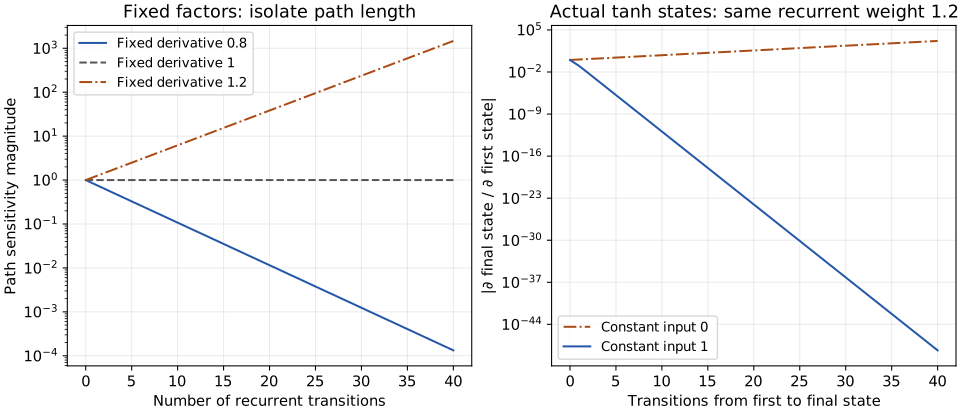
The plots measure a path sensitivity, not the norm of all shared-weight gradients. Later parameter uses can still supply a large total gradient even when a distant signal disappears. Both the actual trajectory and the distance to the supervised output matter.

Clipping limits a large gradient; it cannot recover a lost one

Once BPTT has computed all parameter derivatives, collect them into a single vector \(\mathbf g=\nabla_\theta\mathcal L\) by conceptually flattening and joining the parameter arrays. For a positive threshold \(\tau\), norm clipping gives

\[ \mathbf g_{\mathrm{clip}}= \begin{cases} \mathbf g,&\|\mathbf g\|_2\leq\tau,\\ \displaystyle\tau\frac{\mathbf g}{\|\mathbf g\|_2},&\|\mathbf g\|_2>\tau. \end{cases} \]

A gradient longer than \(\tau\) keeps its direction but has its length reduced. The zero gradient uses the first branch, avoiding division by zero. Apply clipping after backward and before the optimizer step. It can limit a very large gradient from disrupting an update; it cannot reconstruct information that vanished along an earlier path. For ordinary gradient descent, the update length is at most \(\eta\tau\). An adaptive optimizer transforms the gradient further, so that bound does not directly constrain its parameter-step length.

A GRU learns how much to retain and how much to write

The simple cell transforms its old state through the full affine map and activation at every step. A gated recurrent unit (GRU) adds a direct route for retaining old state and learns how much of it to use. A gate is a vector of sigmoid outputs in \((0,1)\), computed from the current observation and previous state. It multiplies matching coordinates; it is neither a fixed hyperparameter nor an on/off instruction.

Write \(\mathbf u_t\) for the retention/update gate, \(\mathbf r_t\) for the reset gate, and \(\widetilde{\mathbf h}_t\) for a candidate state. All have shape \(1\times H\). The state update is

\[ \mathbf h_t=\mathbf u_t\odot\mathbf h_{t-1} +(\mathbf 1-\mathbf u_t)\odot\widetilde{\mathbf h}_t. \]

A coordinate of \(\mathbf u_t\) near one largely retains the corresponding old state; near zero it favors the candidate. For one coordinate, \(u=0.9\), old state \(0.5\), and candidate \(-0.4\) give \(0.9(0.5)+0.1(-0.4)=0.410\). These illustrative values explain the mixture; they are not outputs of a trained model.

To make the gates precise, use the lecture’s PyTorch GRU convention. For \(a\in\{u,r\}\),

\[ \mathbf a_t=\sigma\!\left( \mathbf x_t\mathbf W_{xa}^\top+\mathbf b_{xa} +\mathbf h_{t-1}\mathbf W_{ha}^\top+\mathbf b_{ha}\right). \]

The candidate uses

\[ \begin{aligned} \widetilde{\mathbf h}_t=\tanh\Bigl(&\mathbf x_t\mathbf W_{xn}^\top+\mathbf b_{xn}\\ &+\mathbf r_t\odot(\mathbf h_{t-1}\mathbf W_{hn}^\top+\mathbf b_{hn})\Bigr). \end{aligned} \]

Each input matrix has shape \(H\times D\) and each recurrent matrix \(H\times H\). The sigmoid \(\sigma(v)=1/(1+e^{-v})\) acts coordinatewise. Reset controls how much of the recurrent affine result enters the candidate. In this implementation it acts after that affine operation, including its bias; gating the previous state before multiplying by \(\mathbf W_{hn}\) is generally a different model. PyTorch calls its update gate \(z_t\); we use \(\mathbf u_t\) to preserve \(\mathbf z_t\) for preactivations. Some sources use the opposite mixture convention, so inspect which term receives the named gate.

Holding gate and candidate values fixed, the direct carry derivative is \(\operatorname{diag}(\mathbf u_t)\). That route can avoid repeatedly passing through the candidate’s tanh derivative. However, both gates and candidate depend on the old state: the full Jacobian includes those additional derivatives. A carry gate near one creates a useful route, not a guarantee of stable gradients or successful memory.

An LSTM separates stored memory from the visible state

A long short-term memory (LSTM) cell maintains two vectors: cell storage \(\mathbf c_t\) and visible hidden state \(\mathbf h_t\), each of width \(H\). A forget gate \(\mathbf f_t\) controls retained storage, an input gate \(\mathbf i_t\) controls writing, and an output gate \(\mathbf o_t\) controls exposure of the storage to the hidden state. With candidate \(\widetilde{\mathbf c}_t\),

\[ \begin{aligned} \mathbf c_t&=\mathbf f_t\odot\mathbf c_{t-1} +\mathbf i_t\odot\widetilde{\mathbf c}_t,\\ \mathbf h_t&=\mathbf o_t\odot\tanh(\mathbf c_t). \end{aligned} \]

For the plain modern cell shown in the lecture, without projection or peephole connections, define the three sigmoid gates by

\[ \mathbf a_t=\sigma\!\left( \mathbf x_t\mathbf W_{xa}^\top +\mathbf h_{t-1}\mathbf W_{ha}^\top+\mathbf b_a\right), \qquad a\in\{f,i,o\}, \]

and the candidate by

\[ \widetilde{\mathbf c}_t=\tanh\!\left( \mathbf x_t\mathbf W_{xc}^\top +\mathbf h_{t-1}\mathbf W_{hc}^\top+\mathbf b_c\right). \]

Biases here combine the input and recurrent biases used in PyTorch LSTM. Independent sequences start with both states zero in this example. The external task head reads \(\mathbf h_t\); the internal output gate \(\mathbf o_t\) is a different operation from the head weights \(\mathbf W_o\).

Holding gate and candidate values fixed, the direct cell-storage derivative is \(\operatorname{diag}(\mathbf f_t)\). Retention can therefore travel through products of forget gates instead of the simple RNN’s repeated recurrent-affine-and-tanh transformations. Forget values below one still attenuate a long direct path, and dependencies through \(\mathbf h_{t-1}\) add other paths to the full derivative. LSTM does not promise perfect storage or eliminate all gradient problems.

Table 6: Gated cells change the route by which information is retained. All three still use shared parameters and a recurrent dependency between positions.

Cell	State carried between positions	How the state changes
Simple RNN	\(\mathbf h_t\)	Affine mixing followed by an activation
GRU	\(\mathbf h_t\)	Learned coordinatewise mixture of retained state and candidate
LSTM	\((\mathbf c_t,\mathbf h_t)\)	Separate gated retention, writing, and exposure of storage

Gating changes the computation inside a cell. It does not remove the need to process a unidirectional sequence in order, attach an appropriate task head, or train against a stated objective. The following code makes those boundaries visible.

PyTorch: a recurrent layer and a separate prediction head

PyTorch’s nn.RNN processes a complete sequence using the shared recurrent cell. This short CPU example uses three two-feature observations, hidden width two, tanh, and fixed zero biases. A separate nn.Linear head turns the final state into one regression prediction.

import torch
from torch import nn

torch.manual_seed(6)
B, T, D, H, C = 1, 3, 2, 2, 1
X = torch.tensor([[[0.2, -0.1], [0.0, 0.3], [0.4, 0.1]]])
# X has shape (B, T, D): batch, time, input features.
rnn = nn.RNN(D, H, nonlinearity="tanh", bias=False,
             batch_first=True)
head = nn.Linear(H, C, bias=False)

output, final = rnn(X)       # Initial hidden state defaults to zero.
assert output.shape == (B, T, H)
assert final.shape == (1, B, H)
prediction = head(final[0])  # (B, H) -> (B, C)

target = X.new_tensor([[0.5]])
loss = 0.5 * (prediction - target).square().sum()
rnn.zero_grad(set_to_none=True)
head.zero_grad(set_to_none=True)
loss.backward()             # Computes gradients through all time steps.

for t, row in enumerate(output.detach()[0]):
    print(f"h_{t} = [{row[0].item():#.3g}, {row[1].item():#.3g}]")
print(f"prediction = {prediction.item():.3g}")
print(f"loss = {loss.item():.3g}")

With PyTorch 2.8 on CPU and the seed above, this prints (three significant digits):

h_0 = [0.0128, 0.122]
h_1 = [0.00930, 0.0915]
h_2 = [0.0384, 0.314]
prediction = -0.144
loss = 0.208

The final state is the last displayed row. The head combines its two coordinates into one prediction; comparing that prediction with the target \(0.5\) gives the loss. These are results from the seeded, untrained model, not a fitted forecast.

output contains the hidden state at every position, shape \((B,T,H)\). final contains the final state for each layer and direction. Here there is one layer and one direction, so final[0] selects the final state of each sequence, shape \((B,H)\). batch_first=True changes the sequence layout; it does not change this final-state layout.

The recurrent layer produces representations. The separate head maps the final representation to the task prediction. Applying head(output) would instead produce a prediction at every position, shape \((B,T,C)\), requiring corresponding targets. bias=False matches our fixed-zero-bias example; the activation is now specifically tanh.

The loss retains the factor \(1/2\) and sums over examples and output coordinates, as in the derivation. loss.backward() computes parameter gradients; an optimizer would then update the parameters. Clear .grad buffers before each backward pass unless accumulation is intentional. For norm clipping, insert torch.nn.utils.clip_grad_norm_(list(rnn.parameters()) + list(head.parameters()), max_norm=1.0) after backward and before the optimizer step.

These untrained parameters illustrate the computation. The Week 06 tutorial supplies full learning experiments. Next we will give each word its own positioned representation before attention combines available positions directly.

Words become positioned token representations

We now turn to Transformer models, which use attention to combine information from different sequence positions. Within a layer, positions can be computed together rather than through a recurrent state chain, and distant positions can interact directly. These properties make Transformers useful for constructing contextual representations, although ordinary full attention has a cost that grows quadratically with sequence length.

This chapter studies the Transformer encoder: the part that turns a supplied sequence into representations informed by its available context. Those representations can support tasks such as classifying a sequence or labeling its words. The original Transformer also has a decoder for producing an output sequence; we will not build that decoder here. Our sentence-completion example gives a concrete input and motivating target while we learn the encoder’s machinery. First we must represent token identity and position numerically; then we will build attention and the complete encoder block. See Vaswani et al. (2017), §§3–4 for the original architecture and computational comparison.

Turn the completion into a sequence of token IDs

Return to the sentence we want to complete:

A journey of a thousand miles begins → with a single step.

The supplied prefix has seven words. We want to understand how a model turns those words into numerical representations before it predicts a continuation. Knowing the familiar phrase gives us a target; it does not mean that our small, untrained model can produce it.

A token is one unit in a discrete input sequence. For this example, use a deliberately simple rule: lowercase the words, split at spaces, and omit punctuation. Our input is therefore

a  journey  of  a  thousand  miles  begins

This rule makes one word one token here. Other tokenizers can split words into smaller pieces; the seven-position count belongs to our declared example.

A vocabulary lists the distinct tokens the model can represent. Give each token an integer ID, starting at zero. Include the continuation words now, so the same vocabulary can later describe both supplied words and predicted words. There are six distinct types in the prefix, plus with, single, and step: vocabulary size \(K=9\). No padding, unknown-word, or end-of-sequence token is needed for this fixed example. A more general application would need an explicit policy for words outside its vocabulary.

Table 7: Seven positions select six distinct token types. The two occurrences of a have the same ID, but different positions.

Position \(t\)	Input token	Token ID \(k_t\)
0	a	0
1	journey	1
2	of	2
3	a	0
4	thousand	3
5	miles	4
6	begins	5

An ID is a lookup index, not a measurement. ID 4 does not make miles twice as meaningful as ID 2. The order of vocabulary entries is arbitrary, provided the lookup and output labels agree. Keep three counts separate: \(T=7\) positions, \(K=9\) vocabulary entries, and \(D=5\) representation features.

Look up a five-coordinate embedding for each token

An embedding assigns a real-valued vector to a discrete token. Store those vectors as rows of an embedding table \(\mathbf E_{\mathrm{vocab}}\in\mathbb R^{K\times D}\). The ID selects a row; it is not multiplied into the row. For position \(t\),

\[ \mathbf e_t=\mathbf E_{\mathrm{vocab}}[k_t,:], \qquad \mathbf e_t\in\mathbb R^{1\times D}. \]

The colon means “all feature coordinates.” In a trained model, the embedding table is usually a parameter learned with the rest of the network. For the arithmetic below, choose the explicit, untrained illustrative table in Table 8. Width five keeps every coordinate visible; it is not a claim that five features suffice for real language understanding. We label coordinates by index, without assigning invented meanings such as “distance” or “importance” to them.

Table 8: The illustrative vocabulary embedding table \(\mathbf E_{\mathrm{vocab}}\) has nine rows and five features. Rows are shared by every occurrence of a token.

ID	Token	\(j=0\)	\(j=1\)	\(j=2\)	\(j=3\)	\(j=4\)
0	a	0.2	-0.1	0.4	0	-0.2
1	journey	0.5	0.3	-0.2	0.1	0.4
2	of	-0.1	0.2	0	-0.3	0.1
3	thousand	0.4	-0.4	0.2	0.5	-0.1
4	miles	0.1	0.5	-0.3	0.2	0.3
5	begins	-0.3	0.1	0.5	-0.2	0.2
6	with	0	-0.2	0.1	0.3	-0.4
7	single	0.3	0	-0.1	0.4	0.2
8	step	-0.2	0.4	0.3	-0.1	0.5

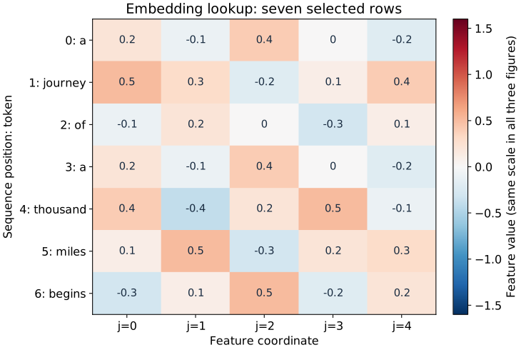
Stack the selected rows in input order to form the sequence embedding matrix \(\mathbf E_{\mathrm{seq}}\in\mathbb R^{7\times5}\). It has one row per occurrence, so the table’s a row is selected twice. For instance,

\[ \mathbf e_0=\mathbf e_3=(0.2,-0.1,0.4,0,-0.2). \]

Figure 4 shows all seven selected rows. Compare the first and fourth rows: their values match exactly. Lookup alone supplies token identity; it has not yet supplied a position-dependent feature or combined information from other words.

Figure 4: Embedding lookup creates seven rows of five features. Both occurrences of a select the same vocabulary row. Values are illustrative and untrained; annotations use three significant digits. Original course calculation.

Supply position as a second vector

A recurrent cell encounters positions through successive state updates. The attention calculation we will build next receives all seven rows together. We therefore supply numerical position information alongside token identity. A positional encoding assigns a vector \(\mathbf p_t\) to position \(t\); a token appearing elsewhere receives a different position vector.

Use fixed sine and cosine functions at several frequencies, following the sinusoidal construction in Vaswani et al. (2017), §3.5. Let \(j=0,\ldots,D-1\) index a feature, and let \(\lfloor j/2\rfloor\) denote the integer part of \(j/2\). Define

\[ \begin{aligned} \omega_j&=10000^{-2\lfloor j/2\rfloor/D},\\ P_{t,j}&= \begin{cases} \sin(t\omega_j),&j\text{ even},\\ \cos(t\omega_j),&j\text{ odd}. \end{cases} \end{aligned} \]

Here \(\omega_j\) is an angular frequency, and the trigonometric functions use radians. Neighboring sine/cosine coordinates share a frequency. With our odd width \(D=5\), the five entries are

\[ \mathbf p_t=\left( \sin t,\ \cos t,\ \sin\frac{t}{10000^{2/5}},\ \cos\frac{t}{10000^{2/5}},\ \sin\frac{t}{10000^{4/5}} \right). \]

The first pair changes quickly over seven positions. The second pair changes more slowly; the final sine changes more slowly still. At position zero, sine is zero and cosine is one, giving \(\mathbf p_0=(0,1,0,1,0)\). At position three,

\[ \mathbf p_3\approx(0.141,-0.990,0.0753,0.997,0.00189). \]

Figure 5 shows the complete \(7\times5\) matrix \(\mathbf P\). These vectors depend on position, not on which word occupies it. Their slow coordinates need not vary greatly within a short prefix; the annotation makes that small variation visible.

Figure 5: Seven positions produce five sinusoidal features each. The first pair varies quickly, while later coordinates change slowly across this short prefix. The final sine is unpaired because the teaching width is odd. Original course calculation.

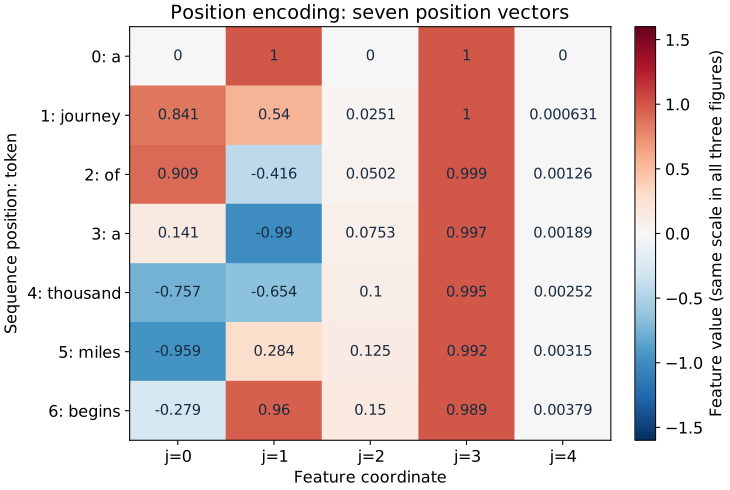
The usual even-width construction has complete sine/cosine pairs. For each complete pair, angle-addition identities express the encoding at \(t+\Delta\) as a linear transformation of the pair at \(t\), with coefficients depending on the offset \(\Delta\). Our width-five example explicitly truncates that construction: coordinate four is an unpaired sine. Do not assume that the same two-coordinate relative-shift relation holds for that last coordinate alone. This choice keeps the requested five-feature arithmetic consistent; the lecture’s paired formula describes the standard even-width case.

Add token identity and position coordinate by coordinate

Both selected embeddings and position vectors have five coordinates. Add their corresponding entries:

\[ \mathbf h_t^{(0)}=\mathbf e_t+\mathbf p_t, \qquad \mathbf H^{(0)}=\mathbf E_{\mathrm{seq}}+\mathbf P \in\mathbb R^{7\times5}. \]

The superscript \((0)\) denotes the input representation before the first encoder layer; it is a depth label, not a power or time step. Capital \(\mathbf H^{(0)}\) stacks the row representations \(\mathbf h_t^{(0)}\) at all seven positions. Addition preserves five features per row; concatenation would instead produce ten and is not the operation used here.

For the first a, at \(t=0\),

\[ \begin{aligned} \mathbf h_0^{(0)} &=(0.2,-0.1,0.4,0,-0.2)+(0,1,0,1,0)\\ &=(0.2,0.9,0.4,1,-0.2). \end{aligned} \]

For the second a, at \(t=3\), the same embedding combines with a different positional vector:

\[ \mathbf h_3^{(0)}\approx(0.341,-1.09,0.475,0.997,-0.198). \]

For example, its first coordinate is \(0.2+\sin 3\approx0.341\). Its second is \(-0.1+\cos 3\approx-1.09\). Figure 6 shows every resulting row. The two a occurrences are now distinct, although their underlying token embedding is still shared. All calculations use full precision; displayed values are rounded only afterward.

Figure 6: Adding position changes the repeated a rows while preserving a seven-by-five shape. Each entry is the corresponding embedding entry plus position entry. These are positioned inputs, before attention has mixed any words. Original course calculation.

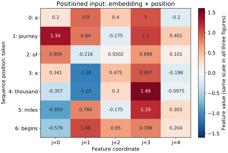
The three heatmaps use the same color scale, so a color has the same numerical meaning before and after addition. The annotations also expose values too small to distinguish by color.

Our example uses unscaled embeddings. The original Transformer multiplies token embeddings by \(\sqrt{D}\) before adding position (Vaswani et al., §3.4). We omit that scaling throughout this teaching example rather than silently changing its numbers. Fixed sinusoidal encodings are also not the only way to represent position; learned position embeddings are another choice.

NotePause and predict: what changed for the second “a”?

The token a occurs at positions zero and three. Which rows are equal before adding position? Which rows differ afterward? Has the word’s embedding been replaced by a second learned embedding?

Reveal the explanation

Both occurrences select the same vocabulary row, so \(\mathbf e_0=\mathbf e_3\). Position supplies \(\mathbf p_0\ne\mathbf p_3\), hence \(\mathbf h_0^{(0)}\ne\mathbf h_3^{(0)}\). There is still one shared embedding for a; its two occurrences have different positioned representations. Neither has yet received information from the other words through attention.

What this matrix is ready to do—and what it has not done

Table 9: Vocabulary size, sequence length, and model width govern different axes. Adding position preserves the sequence shape.

Object	Shape	What its rows describe
\(\mathbf E_{\mathrm{vocab}}\)	\(9\times5\)	One embedding for each vocabulary type
\(\mathbf E_{\mathrm{seq}}\)	\(7\times5\)	Embeddings selected for input occurrences
\(\mathbf P\)	\(7\times5\)	Position information for those occurrences
\(\mathbf H^{(0)}\)	\(7\times5\)	Input occurrences with identity and position combined

We have converted a supplied prefix into seven positioned feature rows. This is the input to our attention walkthrough. It is not seven predicted words and contains no vocabulary probabilities. At this stage, each row depends only on its selected embedding and position; attention will later let a row use information from permitted source positions.

A next-word task will ultimately need a vocabulary head: a map from a contextual feature row of width five to nine scores, one per vocabulary token, followed by a probability calculation. Its stored weight shape would be \(K\times D=9\times5\). That task head is distinct from the embedding table, whose stored shape is \(K\times D\) too but whose operation is lookup. Matching shapes do not make the two operations interchangeable.

The desired first continuation token is with, ID 6. We have included it in the vocabulary, but have not trained a representation or head to predict it. We will keep this exact token order, embedding table, and position rule for the attention calculations in the next sections.

One attention head, one operation at a time

What should one position read from the others?

The positioned matrix \(\mathbf H^{(0)}\) gives each word its own five-feature row. How can the row for begins use information from journey or miles? Self-attention builds a new row by combining information from positions in the same supplied sequence. A query at a position determines how strongly each permitted source contributes. The source can include the query’s own position.

An attention head is one such matching-and-mixing computation with its own projection parameters. We will follow one head with query/key width \(d_k=3\) and value width \(d_v=3\). Its three output features are an intermediate representation. Multiple heads and the return to model width five come in the next section.

For this standalone calculation, use \(\mathbf H^{(0)}\) directly, with the full-precision values from the previous section. We omit projection biases, normalization, and dropout to expose the attention operations. When we later insert attention into the complete pre-norm encoder, normalization will change its input, so those numerical projections must be recomputed.

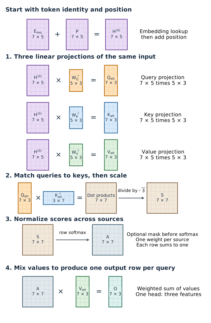
Before following the numbers, Figure 7 shows the complete route. Embedding lookup supplies token features, and adding positional encoding produces the purple \(7\times5\) input. The attention head then applies three linear maps: orange for queries, blue for keys, and green for values. It multiplies queries by transposed keys, divides the scores by \(\sqrt3\), applies softmax across each row, and multiplies the resulting weights by the values. The output has one three-feature row for each of the seven input positions. We will unpack those operations in that order. Position is added before this standalone head; it is not added separately inside each projection.

Figure 7: The full route from embeddings and position to one attention head’s output. Purple input matrices multiply orange query, blue key, and green value projection matrices; matching, scaling, row softmax, and value mixing follow. Rectangle widths and heights reflect column and row counts using the same unit size. Original course diagram.

Give the same input three different roles

Project the input along three branches, shown in Figure 7:

• A query \(\mathbf q_t\) represents what position \(t\) uses to match sources.
• A key \(\mathbf k_j\) represents what source position \(j\) uses for that match.
• A value \(\mathbf v_j\) supplies the features that will actually be combined.

These names describe computational roles; they do not assign a particular linguistic meaning to an untrained coordinate. Queries and keys together determine the weights, while values supply the content. The source index \(j\) ranges over sequence positions, not vocabulary IDs or feature coordinates.

We conceptually reuse the same input on three branches; there is no mathematical requirement to allocate three physical copies. Each map is shared across all seven rows, just as a linear layer uses the same weights for every example. Choose the following sparse, untrained parameters to keep the arithmetic readable. Under our output-by-input storage convention, \(\mathbf W_Q,\mathbf W_K,\mathbf W_V\) are \(3\times5\). The matrices multiplied on the right are their \(5\times3\) transposes:

\[ \mathbf W_Q^\top= \begin{bmatrix} 1&0&0\\0&1&0\\0&0&1\\0&0&0\\0&0&0 \end{bmatrix}, \qquad \mathbf W_K^\top= \begin{bmatrix} \tfrac12&0&0\\0&1&0\\0&0&\tfrac12\\\tfrac12&0&0\\0&0&\tfrac12 \end{bmatrix}. \]

\[ \mathbf W_V^\top= \begin{bmatrix} 1&0&0\\0&0&0\\0&1&0\\0&0&\tfrac12\\0&0&\tfrac12 \end{bmatrix}. \]

The original attention paper names the right-multiplication matrices directly. Our transpose convention preserves the stored orientation used earlier in this course; the multiplication itself is the same.

\[ \begin{aligned} \mathbf Q_{\mathrm{att}}&=\mathbf H^{(0)}\mathbf W_Q^\top,\\ \mathbf K_{\mathrm{att}}&=\mathbf H^{(0)}\mathbf W_K^\top,\\ \mathbf V_{\mathrm{att}}&=\mathbf H^{(0)}\mathbf W_V^\top. \end{aligned} \]

Each multiplication has shape \((7\times5)(5\times3)=7\times3\). We use subscripts “att” to distinguish the key matrix from vocabulary size \(K=9\). For an input row \((h_{t,0},h_{t,1},h_{t,2},h_{t,3},h_{t,4})\) at position \(t\), these specific maps give

\[ \begin{aligned} \mathbf q_t&=(h_{t,0},h_{t,1},h_{t,2}),\\ \mathbf k_t&=\bigl((h_{t,0}+h_{t,3})/2,\ h_{t,1},\ (h_{t,2}+h_{t,4})/2\bigr),\\ \mathbf v_t&=\bigl(h_{t,0},\ h_{t,2},\ (h_{t,3}+h_{t,4})/2\bigr). \end{aligned} \]

For example, the first a row is \((0.2,0.9,0.4,1,-0.2)\), so its key is \((0.6,0.9,0.1)\) and its value is \((0.2,0.4,0.4)\). The full projected arrays are below. These deliberately sparse maps illustrate the operation; a trained projection can use every input feature in every output feature.

Table 10: All seven query rows for this one head. Values are rounded after full-precision calculation.

Position: token	Feature 0	Feature 1	Feature 2
0: a	0.2	0.9	0.4
1: journey	1.34	0.84	-0.175
2: of	0.809	-0.216	0.0502
3: a	0.341	-1.09	0.475
4: thousand	-0.357	-1.05	0.3
5: miles	-0.859	0.784	-0.175
6: begins	-0.579	1.06	0.65

Table 11: All seven key rows for this one head. Values are rounded after full-precision calculation.

Position: token	Feature 0	Feature 1	Feature 2
0: a	0.6	0.9	0.1
1: journey	1.22	0.84	0.113
2: of	0.754	-0.216	0.0757
3: a	0.669	-1.09	0.139
4: thousand	0.569	-1.05	0.101
5: miles	0.167	0.784	0.0642
6: begins	0.105	1.06	0.427

Table 12: All seven value rows for this one head. Values are rounded after full-precision calculation.

Position: token	Feature 0	Feature 1	Feature 2
0: a	0.2	0.4	0.4
1: journey	1.34	-0.175	0.75
2: of	0.809	0.0502	0.4
3: a	0.341	0.475	0.4
4: thousand	-0.357	0.3	0.699
5: miles	-0.859	-0.175	0.748
6: begins	-0.579	0.65	0.496

Follow the “begins” query through seven matches

Take position \(t=6\), begins. Its query is

\[ \mathbf q_6\approx(-0.579,1.06,0.650). \]

To score source \(j=0\), the first a, take the dot product with \(\mathbf k_0=(0.6,0.9,0.1)\). Multiply corresponding features and add:

\[ \begin{aligned} \mathbf q_6\mathbf k_0^\top &=q_{6,0}k_{0,0}+q_{6,1}k_{0,1}+q_{6,2}k_{0,2}\\ &\approx(-0.579)(0.6)+(1.06)(0.9)+(0.650)(0.1)\\ &\approx0.672. \end{aligned} \]

The final value is rounded from the full-precision dot product; recomputing with only displayed rounded inputs may differ slightly. A dot product is a matching score, not a probability. It depends on vector lengths as well as directions, so it is generally not cosine similarity.

Repeat the calculation with each of the seven keys, then divide each result by \(\sqrt{d_k}=\sqrt3\):

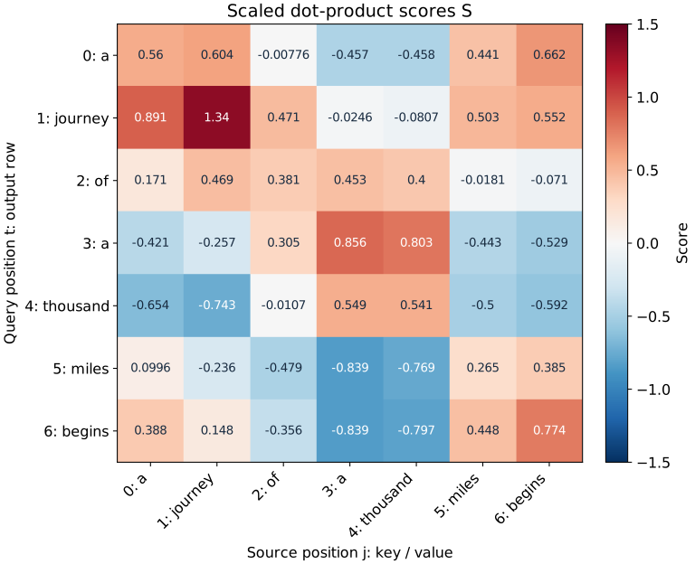
\[ S_{6j}=\frac{\mathbf q_6\mathbf k_j^\top}{\sqrt3}, \qquad S_{60}\approx\frac{0.672}{\sqrt3}\approx0.388. \]

The scale uses the query/key feature width, not the number of words or vocabulary size. Under the motivating assumption of independent zero-mean, unit-variance query/key coordinates, an unscaled dot product has variance \(d_k\); dividing by \(\sqrt{d_k}\) gives variance one. This helps avoid very large scores that make softmax concentrate sharply. It is a scale choice, not a guarantee that actual learned queries meet those assumptions. This is the scaled dot-product construction of Vaswani et al. (2017), §3.2.1.

Table 13: The begins query scores all seven supplied sources; softmax normalizes this one row across sources.

Source \(j\): token	Raw dot product	\(S_{6j}\)	\(A_{6j}\)
0: a	0.672	0.388	0.185
1: journey	0.257	0.148	0.146
2: of	-0.617	-0.356	0.0881
3: a	-1.45	-0.839	0.0544
4: thousand	-1.38	-0.797	0.0567
5: miles	0.776	0.448	0.197
6: begins	1.34	0.774	0.273

Normalize across sources, not across features

For one query, convert its seven scaled scores into seven nonnegative weights using softmax:

\[ A_{6j}=\frac{\exp(S_{6j})}{\sum_{r=0}^{6}\exp(S_{6r})}. \]

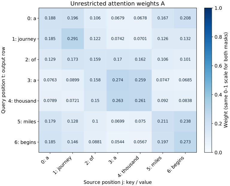
The denominator adds over source positions \(r\). Each query has its own denominator. Its weights sum to one, and a larger score receives a larger weight. Changing one source score changes the other normalized weights too.

For numerical stability, subtract the row maximum \(m_6=\max_r S_{6r}\) before exponentiating:

\[ A_{6j}=\frac{\exp(S_{6j}-m_6)}{\sum_{r=0}^{6}\exp(S_{6r}-m_6)}. \]

The common factor \(\exp(-m_6)\) cancels, so this is the same distribution. The largest exponent is now zero, avoiding overflow from large positive scores. Using the values in Table 13 gives

\[ \mathbf A_{6,:}\approx (0.185,0.146,0.0881,0.0544,0.0567,0.197,0.273). \]

These are weights over the seven supplied occurrences. They are not probabilities for nine possible next words. Their full-precision sum is one; a sum of rounded values may differ slightly.

Use each weight to scale an entire value vector

One scalar weight \(A_{6j}\) multiplies all three features in \(\mathbf v_j\). Add the seven weighted vectors to obtain the output row \(\mathbf o_6\):

\[ \mathbf o_6=\sum_{j=0}^{6}A_{6j}\mathbf v_j. \]

For the first source, the contribution is

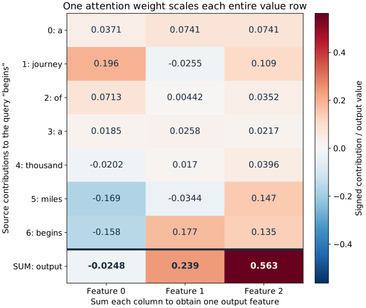
\[ A_{60}\mathbf v_0 \approx0.185\,(0.2,0.4,0.4) \approx(0.0371,0.0741,0.0741). \]

Table 14 lists all seven contributions. Sum its first feature column for output feature zero, its second for feature one, and its third for feature two. The result is

\[ \mathbf o_6\approx(-0.0248,0.239,0.563). \]

Table 14: Each source contributes its value vector multiplied by one scalar attention weight. Sum each feature column to obtain the begins output row.

Source \(j\): token	Contribution 0	Contribution 1	Contribution 2
0: a	0.0371	0.0741	0.0741
1: journey	0.196	-0.0255	0.109
2: of	0.0713	0.00442	0.0352
3: a	0.0185	0.0258	0.0217
4: thousand	-0.0202	0.017	0.0396
5: miles	-0.169	-0.0344	0.147
6: begins	-0.158	0.177	0.135

Figure 8 makes the same sum visible: each of the first seven rows is one weighted value vector, and each column is one feature. The separate bottom row adds the entries above it. Read downward within a column, not across words as a time series. Attention weights are nonnegative, but value coordinates can be negative, so contributions can cancel. The output is a weighted average of value vectors; it is not an average of word IDs, keys, or predicted token probabilities.

Figure 8: For the query begins, each source contributes three weighted value features. The separated bottom row contains the three column sums: the output representation for begins. Blue and red distinguish negative and positive values, so cancellation is visible. Original course calculation.

Stack the same calculation for all seven queries

Nothing about the matching rule is special to position six. Repeat it for each query row, or express all rows in matrix form:

\[ \begin{aligned} \mathbf S&=\frac{\mathbf Q_{\mathrm{att}}\mathbf K_{\mathrm{att}}^\top}{\sqrt3} \in\mathbb R^{7\times7},\\ \mathbf A&=\operatorname{softmax}_{\mathrm{rows}}(\mathbf S) \in\mathbb R^{7\times7},\\ \mathbf O&=\mathbf A\mathbf V_{\mathrm{att}} \in\mathbb R^{7\times3}. \end{aligned} \]

The score product is \((7\times3)(3\times7)\). Its row \(t\) belongs to query \(t\); its column \(j\) belongs to source \(j\). Row softmax leaves both axes in place. The value product is \((7\times7)(7\times3)\): its shared dimension sums over source positions, leaving one three-feature output per query.

Figure 9 and Figure 10 show the full score and weight matrices. Read the last row to find the earlier begins walkthrough. Read another row to see that a different query induces different weights, even though it reads the same keys and values.

Figure 9: Each query scores every source key. Rows identify queries and columns identify sources; the last row is the begins calculation. Scores can be negative and are not normalized probabilities. Original course calculation.

Figure 10: Row softmax turns each query’s seven scores into weights summing to one. All seven source positions are visible in this unrestricted calculation. Original course calculation.

Table 15: All seven output rows for this one head. Values are rounded after full-precision calculation.

Position: token	Feature 0	Feature 1	Feature 2
0: a	0.122	0.205	0.567
1: journey	0.342	0.15	0.579
2: of	0.237	0.206	0.556
3: a	0.16	0.262	0.541
4: thousand	0.103	0.268	0.543
5: miles	-0.0337	0.228	0.563
6: begins	-0.0248	0.239	0.563

The parameters are shared maps, but \(\mathbf A\) is computed from this input. It is not a permanently learned table of seven-by-seven weights. This one head returns \(7\times3\) features; it has not yet returned the encoder’s width-five representation or made a vocabulary prediction.

NotePause and predict: what do the seven weights multiply?

For the begins query, softmax returns seven weights. Does each weight correspond to an input feature, a vocabulary word, or a source position? Which vector does \(A_{62}\) multiply, and how many features remain in the result?

Reveal the explanation

Each weight corresponds to a source position. \(A_{62}\) multiplies the whole three-feature value vector at position two, of. Adding the seven weighted value vectors leaves three features in the output row. Softmax normalizes over the seven sources; it does not normalize over the three value features or the nine vocabulary entries.

Change visibility with a mask

Our first calculation encodes the complete supplied prefix: every row can use every supplied word. Such unrestricted visibility is appropriate when the entire input is available for the task. A different task may require each row to use only its own prefix, for example when predictions at earlier positions must not see later words.

A causal mask permits source \(j\) when \(j\leq t\) and excludes it when \(j>t\). Add a mask to the scores before softmax:

\[ M_{tj}=\begin{cases}0,&j\leq t,\\-\infty,&j>t,\end{cases} \qquad \mathbf A^{\mathrm{causal}} =\operatorname{softmax}_{\mathrm{rows}}(\mathbf S+\mathbf M). \]

Excluded sources get weight zero because \(\exp(-\infty)=0\). Allowed sources are renormalized to sum to one. Simply zeroing some already-normalized weights would leave the wrong total and is not the same operation. Every query here includes itself, so no row is fully masked; softmax on an all-\(-\infty\) row would be undefined.

At begins, \(t=6\), both rules allow all seven supplied sources: their last rows are identical. Look instead at journey, \(t=1\), in Table 16. Its causal weights are approximately \((0.389,0.611,0,0,0,0,0)\), because only the first a and journey are available.

Table 16: The journey query at position one distinguishes the visibility rules: causal attention renormalizes over positions zero and one only.

Source \(j\): token	Unrestricted \(A_{1j}\)	Causal \(A_{1j}\)
0: a	0.185	0.389
1: journey	0.291	0.611
2: of	0.122	0
3: a	0.0742	0
4: thousand	0.0701	0
5: miles	0.126	0
6: begins	0.132	0

Figure 11: A causal mask removes future sources before normalization. Crosses mark exact zero weights at excluded positions; each allowed row still sums to one. The last row matches unrestricted attention. Original course calculation, using the same weight color scale.

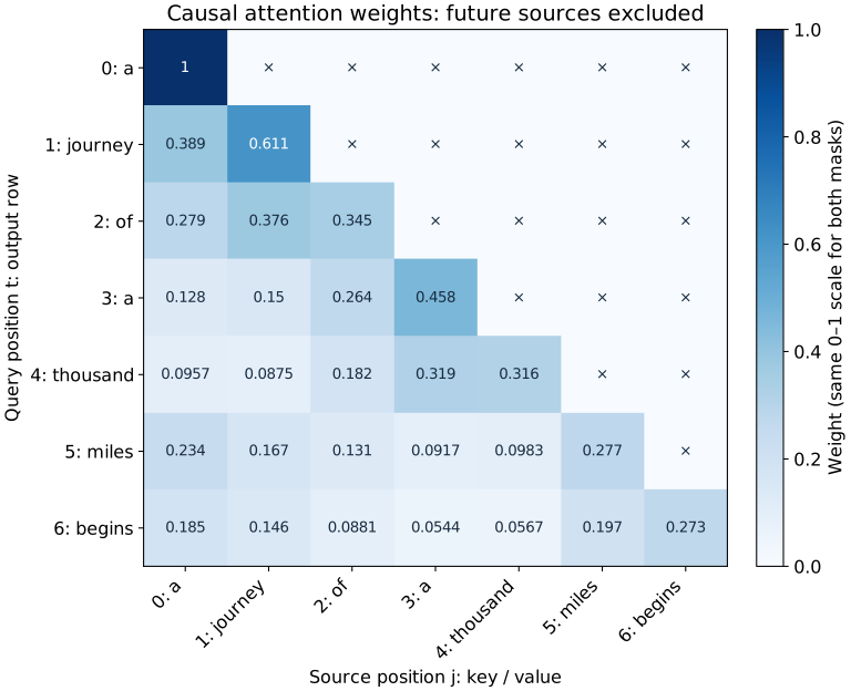
The masked head output is \(\mathbf O^{\mathrm{causal}}=\mathbf A^{\mathrm{causal}}\mathbf V_{\mathrm{att}}\). For this standalone head, changing an input row after position one cannot change the causal output at position one: it cannot change that query or any permitted source key/value. The same change can affect the unrestricted output. In a full model, the information boundary must hold in all earlier layers too; a late mask cannot undo future information already mixed into an input row.

We will use unrestricted attention for our encoder walkthrough on the supplied prefix. The completion remains a motivation, not a demonstration of an autoregressive decoder. We now have one checked head; the next section will give another head its own projection maps, join their output features, and return to width five.

Multiple heads return a contextual representation of the same width

One head chooses a distribution over source positions and mixes three value features using that distribution. A second head can choose another distribution and extract another set of features. Multiple heads give each query several separately computed views of the same context. They read the same input; they do not process consecutive chunks of the sentence.

We retain \(T=7\), model width \(D=5\), and the first head exactly as calculated above. Add a second head with query/key width \(d_k=3\) and value width \(d_v=3\). Both heads use unrestricted visibility over the supplied prefix. All maps below are illustrative, untrained parameters; we continue to omit biases and dropout.

Two heads, two sets of projection parameters

The superscript \([i]\) labels a head, not a time step or encoder layer. For \(i=1,2\),

\[ \begin{aligned} \mathbf Q_{\mathrm{att}}^{[i]}&=\mathbf H^{(0)}(W_Q^{[i]})^\top,\\ \mathbf K_{\mathrm{att}}^{[i]}&=\mathbf H^{(0)}(W_K^{[i]})^\top,\\ \mathbf V_{\mathrm{att}}^{[i]}&=\mathbf H^{(0)}(W_V^{[i]})^\top,\\ \mathbf A^{[i]}&=\operatorname{softmax}_{\mathrm{row}}\!\left( \frac{\mathbf Q_{\mathrm{att}}^{[i]}(\mathbf K_{\mathrm{att}}^{[i]})^\top}{\sqrt{3}}\right),\\ \mathbf O^{[i]}&=\mathbf A^{[i]}\mathbf V_{\mathrm{att}}^{[i]}. \end{aligned} \]

The first head’s maps are the \(W_Q,W_K,W_V\) from the single-head walkthrough. The second uses

\[ W_Q^{[2]}=\begin{bmatrix}0&0&0&1&0\\0&0&0&0&1\\0.5&0.5&0&0&0\end{bmatrix},\qquad W_K^{[2]}=\begin{bmatrix}0&0&0&1&0\\0&0&1&0&0\\0&0.5&0&0&0.5\end{bmatrix}, \]

\[ W_V^{[2]}=\begin{bmatrix}0&1&0&0&0\\0&0&0&1&0\\0.5&0&0&0&0.5\end{bmatrix}. \]

Each stored map is \(3\times5\), so its right-multiplication transpose is \(5\times3\). Both heads project the full five-feature input. The sparse entries make hand calculation easy; head 2 is not restricted to a predefined second half of the input.

For the begins row, head 2 therefore constructs

\[ \begin{aligned} \mathbf q_6^{[2]}&=(h_{6,3}^{(0)},\;h_{6,4}^{(0)},\;0.5h_{6,0}^{(0)}+0.5h_{6,1}^{(0)}) \\&\approx(0.789,\;0.204,\;0.240),\\ \mathbf v_6^{[2]}&=(h_{6,1}^{(0)},\;h_{6,3}^{(0)},\;0.5h_{6,0}^{(0)}+0.5h_{6,4}^{(0)}) \\&\approx(1.06,\;0.789,\;-0.188). \end{aligned} \]

It repeats the score, scaling, and row-softmax operations from the single-head walkthrough using its own keys. Table 17 compares the resulting mixtures for the same query. Each column of weights here sums to one because it displays one query’s complete source distribution from one head. We do not normalize the two heads together.

Table 17: Two independently normalized source mixtures for the same begins query. Both heads can read all seven sources.

Source	Head 1 weight	Head 2 weight
0: a	0.185	0.147
1: journey	0.146	0.149
2: of	0.0881	0.116
3: a	0.0544	0.129
4: thousand	0.0567	0.16
5: miles	0.197	0.154
6: begins	0.273	0.143

The second head assigns a more even distribution in this particular example. That follows from these fixed numbers; it is not evidence that a trained head has discovered a grammatical role. Separate parameters allow different mixtures, but do not force every head to become different or useful (Vaswani et al., §3.2.2).

For begins, the two weighted sums are

\[ \mathbf o_6^{[1]}\approx(-0.0248,\;0.239,\;0.563),\qquad \mathbf o_6^{[2]}\approx(0.196,\;1.06,\;0.0863). \]

The values differ because both the source weights and the value projections differ. Coordinate zero in one head need not mean the same thing as coordinate zero in another. The complete outputs are available below; the first table reproduces the previous section’s one-head result.

Inspect all seven output rows from both heads

Table 18: Head 1 output rows. The three feature axes belong to this head; equal coordinate indices across heads need not have equal meaning.

Position: token	Feature 0	Feature 1	Feature 2
0: a	0.122	0.205	0.567
1: journey	0.342	0.15	0.579
2: of	0.237	0.206	0.556
3: a	0.16	0.262	0.541
4: thousand	0.103	0.268	0.543
5: miles	-0.0337	0.228	0.563
6: begins	-0.0248	0.239	0.563

Table 19: Head 2 output rows. The three feature axes belong to this head; equal coordinate indices across heads need not have equal meaning.

Position: token	Feature 0	Feature 1	Feature 2
0: a	0.277	1.06	0.104
1: journey	0.382	1.05	0.0938
2: of	0.218	1.05	0.0923
3: a	0.0352	1.09	0.0776
4: thousand	-0.0919	1.12	0.0523
5: miles	0.0969	1.08	0.0689
6: begins	0.196	1.06	0.0863

Join features without joining positions

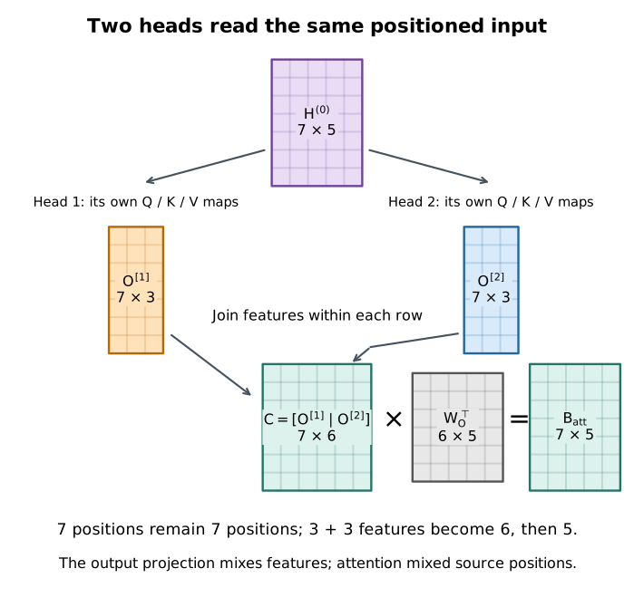
Figure 12 follows both heads through concatenation and projection. Concatenation places the two output vectors side by side within each query row:

\[ \mathbf C=[\mathbf O^{[1]}\mid\mathbf O^{[2]}]\in\mathbb R^{7\times6},\qquad \mathbf c_6\approx(-0.0248,\;0.239,\;0.563,\;0.196,\;1.06,\;0.0863). \]

The first three columns belong to head 1; the next three belong to head 2. Row six still describes begins. Concatenating along the position axis would produce fourteen rows and would be a different operation. We also do not add or average the two head outputs: keeping their coordinates separate lets the next map choose how to combine them.

Figure 12: Two heads read the same seven-by-five input. Their seven-by-three outputs concatenate across features to seven-by-six, then multiply a six-by-five output projection to produce seven-by-five. Positions remain aligned throughout. Original course diagram.

A linear output projection returns to model width

A learnable projection combines the six head features into five model features. We store \(W_O\in\mathbb R^{5\times6}\), so

\[ \mathbf B_{\mathrm{att}}=\mathbf C W_O^\top\in\mathbb R^{7\times5},\qquad W_O=\begin{bmatrix} 1&0&0&0.5&0&0\\ 0&1&0&0&0.5&0\\ 0&0&1&0&0&0.5\\ 0.5&0&0&0&1&0\\ 0&0.5&0&1&0&0 \end{bmatrix}. \]

Here \(\mathbf B_{\mathrm{att}}\) names the attention branch output, which will enter the encoder in the next section. Uppercase \(O\) in \(W_O\) distinguishes this projection from the task readout \(W_o\). This projection mixes features within each row; the attention matrices already performed the mixing across source positions.

For example, the first output feature for begins is

\[ B_{\mathrm{att},6,0}=c_{6,0}+0.5c_{6,3} \approx-0.0248+0.5(0.196)\approx0.0732. \]

The approximation is displayed to three significant digits; the calculation uses the unrounded values. The full row is

\[ \mathbf b_{\mathrm{att},6}\approx(0.0732,\;0.768,\;0.606,\;1.05,\;0.315). \]

Table 20: All seven attention-branch outputs after concatenation and the output projection. These are five-feature representations, not vocabulary probabilities or complete encoder outputs.

Position: token	Feature 0	Feature 1	Feature 2	Feature 3	Feature 4
0: a	0.26	0.736	0.619	1.12	0.379
1: journey	0.533	0.672	0.626	1.22	0.457
2: of	0.346	0.733	0.602	1.17	0.32
3: a	0.178	0.805	0.58	1.17	0.166
4: thousand	0.057	0.826	0.569	1.17	0.0421
5: miles	0.0147	0.767	0.598	1.06	0.211
6: begins	0.0732	0.768	0.606	1.05	0.315

Table 21: Shape ledger for two width-three heads and a width-five attention branch. The seven positions are preserved at every representation stage.

Stage	Shape	What changes
Positioned input \(\mathbf H^{(0)}\)	\(7\times5\)	Starting representation
Each head’s queries, keys, values	\(7\times3\)	Its own projected features
Each head’s attention weights	\(7\times7\)	Distribution over sources for every query
Each head’s output \(\mathbf O^{[i]}\)	\(7\times3\)	Context mixed within that head
Concatenated outputs \(\mathbf C\)	\(7\times6\)	Two feature sets kept side by side
Output right multiplier \(W_O^\top\)	\(6\times5\)	Map from joined features to model features
Attention branch \(\mathbf B_{\mathrm{att}}\)	\(7\times5\)	Contextual features at the original model width

How this teaching example relates to standard implementations

The usual Transformer convention chooses \(d_k=d_v=D/N_{\mathrm{head}}\), so all head outputs together have width \(D\). The output projection then maps \(D\) features to \(D\) features; it still learns how to mix the heads even though the width is unchanged.

Our deliberately small example uses \(D=5\) and two width-three heads, giving a joined width of six. The attention equations permit this choice. However, PyTorch’s standard nn.MultiheadAttention splits embed_dim equally across heads, so embed_dim=5, num_heads=2 is unsupported. Reproducing this exact example requires explicit \(5\to3\) query/key/value linear maps for each head, the attention operations, feature concatenation, and a \(6\to5\) output linear map (PyTorch 2.8 documentation). Choosing a model width divisible by the number of heads permits the usual module.

We now have seven contextual rows with five features each. These are not generated words or vocabulary probabilities. They are also not yet complete encoder outputs: the next section will place this attention branch inside a block with normalization, residual additions, and a position-wise MLP. In that pre-norm block, attention will receive normalized inputs, so its numerical outputs must be recomputed.

Inside a complete Transformer encoder

Attention lets each word read from other words. An encoder block also needs a way to preserve its incoming representation, transform the gathered features nonlinearly, and keep the inputs to those transformations on a controlled scale. A Transformer encoder combines these jobs using attention, LayerNorm, residual additions, and a position-wise multilayer perceptron (MLP).

Figure 13 connects the entire route: token IDs select embeddings, position vectors are added once, the positioned rows pass through the encoder stack, and a separate task head reads its final representations. The expanded block shows both residual paths; the repetition box repeats that whole block, not only attention. The dashed boundary identifies the encoder after input preparation. The task head lies outside it and will be specified in the next section.

Figure 13: The full pre-norm encoder architecture, from token IDs and positional information to stacked blocks, final normalization, and contextual features. One block is expanded; N_layers counts all blocks, including that one. The separate task head determines predictions. Here T = 7 and D = 5; the numerical walkthrough uses one block, two width-three heads, and F = 4. Original course diagram following the lecture’s visual style.

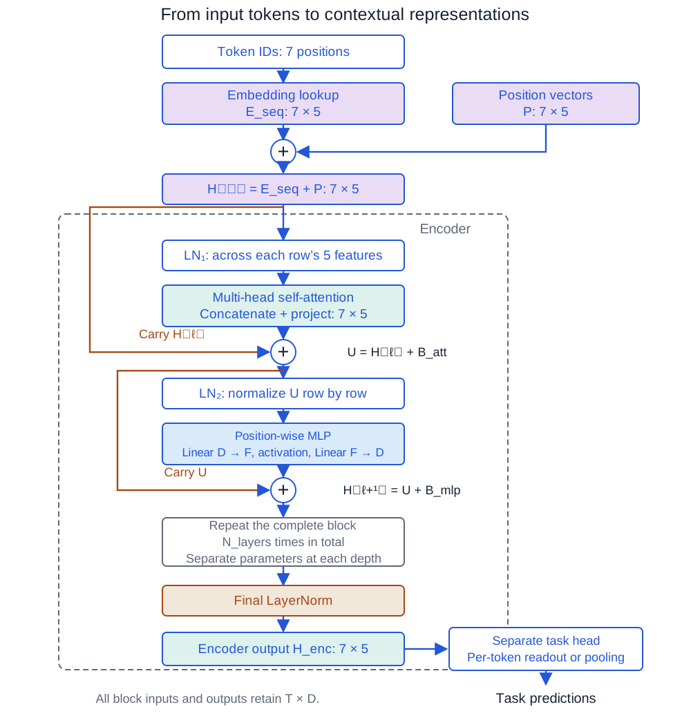
We will assemble the lecture’s pre-norm block: normalize the input to each transformation branch, then add the branch result to a bypass. We retain the same seven positions, five model features, two width-three heads, and attention parameters. The numerical example uses one block, an MLP hidden width \(F=4\), and ReLU. Attention biases and dropout remain omitted; MLP biases are included explicitly. All parameters remain illustrative and untrained.

Read the block as two updates to the representation

For encoder depth \(\ell\), the block computes

\[ \begin{aligned} \mathbf X&=\operatorname{LN}_1(\mathbf H^{(\ell)}),\\ \mathbf B_{\mathrm{att}}&=\operatorname{MHA}(\mathbf X),\\ \mathbf U&=\mathbf H^{(\ell)}+\mathbf B_{\mathrm{att}},\\ \mathbf R&=\operatorname{LN}_2(\mathbf U),\\ \mathbf B_{\mathrm{mlp}}&=\operatorname{MLP}(\mathbf R),\\ \mathbf H^{(\ell+1)}&=\mathbf U+\mathbf B_{\mathrm{mlp}}. \end{aligned} \]

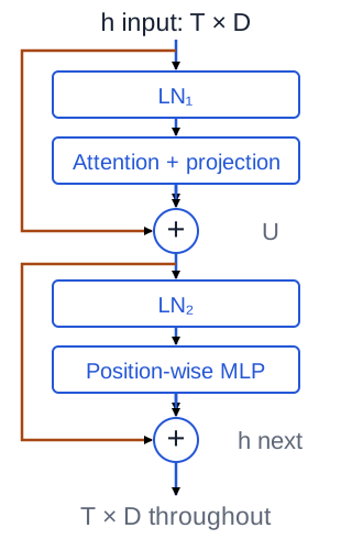
Here \(\operatorname{MHA}\) includes both heads, feature concatenation, and the output projection from the multi-head walkthrough. Every matrix above has shape \(7\times5\). Figure 14 isolates the two bypasses. The first addition preserves the block input \(\mathbf H^{(\ell)}\); the second preserves the intermediate result \(\mathbf U\). Neither addition carries the normalized branch input. These are residual updates of the same kind introduced in the Week 05 chapter.

Figure 14: The lecture’s pre-norm block schematic: LN₁ precedes attention and its output projection; the first bypass carries the block input to the first addition. LN₂ precedes the MLP; the second bypass carries U to the second addition. Here T = 7 and D = 5. Original course figure reused from the Week 06 lecture.

Table 22: New notation for the encoder block. Each LayerNorm has its own scale and shift parameters.

Symbol	Meaning in this block
\(\ell\)	Encoder depth; independent of token position \(t\) and head index \([i]\)
\(\mathbf X\), \(\mathbf R\)	Normalized inputs to attention and the MLP
\(\mathbf U\)	Representation after the first residual addition
\(\mathbf B_{\mathrm{att}}\), \(\mathbf B_{\mathrm{mlp}}\)	Outputs of the two transformation branches
\(F\)	MLP hidden width, four in this example
\(\boldsymbol\gamma\), \(\boldsymbol\beta\)	Learned feature scales and shifts of one LayerNorm
\(\epsilon\)	Positive denominator stabilizer, \(10^{-5}\) here

LayerNorm looks across features within one word

Figure 15 separates the axes of the three operations: attention combines source positions, while LayerNorm and the shared MLP operate within each row.

Figure 15: Attention mixes positions, LayerNorm computes statistics across a row’s features, and the MLP transforms each row using shared weights. The three-row, four-feature grids are schematic; our numerical example remains seven-by-five. Original course figure reused from the Week 06 lecture.

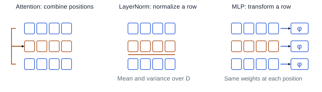
For a row \(\mathbf h_t\in\mathbb R^5\), LayerNorm first calculates its mean and population variance across the five features:

\[ \mu_t=\frac15\sum_{c=0}^4 h_{t,c},\qquad \sigma_t^2=\frac15\sum_{c=0}^4(h_{t,c}-\mu_t)^2. \]

Then, for feature \(c\),

\[ \operatorname{LN}(\mathbf h_t)_c =\gamma_c\frac{h_{t,c}-\mu_t}{\sqrt{\sigma_t^2+\epsilon}}+\beta_c. \]

Subtracting the mean centers the row; division controls its scale. The learned \(\gamma_c\) and \(\beta_c\) let the model adjust each resulting feature. One parameter vector is shared across positions, but each position supplies its own statistics. \(\operatorname{LN}_1\) and \(\operatorname{LN}_2\) have separate trainable parameters even when they start with equal values.

For our hand calculation, both use \(\boldsymbol\gamma=(1,1,1,1,1)\) and \(\boldsymbol\beta=(0,0,0,0,0)\). These are parameter values, not a requirement to freeze them. With these values the normalized row has zero mean and variance \(\sigma_t^2/(\sigma_t^2+\epsilon)\), slightly below one. A constant row has zero centered features, and therefore produces \(\boldsymbol\beta\); \(\epsilon\) keeps the denominator nonzero.

LayerNorm does not average across words or examples in a batch. For shape \((B,T,D)\), nn.LayerNorm(D) normalizes the last, feature axis independently for each example and position. It uses the current row’s statistics in both training and inference rather than BatchNorm’s running statistics (PyTorch 2.8 LayerNorm documentation). This choice also means normalization itself does not move information between token positions.

For begins, the positioned input is

\[ \mathbf h_6^{(0)}\approx(-0.579,\;1.06,\;0.650,\;0.789,\;0.204). \]

Its mean is \(\mu_6\approx0.425\), and its variance is \(\sigma_6^2\approx0.329\). Normalizing its first feature gives

\[ X_{6,0}=\frac{h_{6,0}^{(0)}-\mu_6}{\sqrt{\sigma_6^2+10^{-5}}} \approx-1.75. \]

The entire normalized row is \(\mathbf x_6\approx(-1.75,1.11,0.393,0.635,-0.385)\). Approximate inputs here explain the arithmetic; all subsequent calculations use unrounded values.

Recompute attention, then add the original input

In the multi-head walkthrough, the two heads read \(\mathbf H^{(0)}\). Inside this block, they read \(\mathbf X=\operatorname{LN}_1(\mathbf H^{(0)})\). For each head, recompute

\[ \mathbf Q_{\mathrm{att}}^{[i]}=\mathbf X(W_Q^{[i]})^\top,\qquad \mathbf K_{\mathrm{att}}^{[i]}=\mathbf X(W_K^{[i]})^\top, \]

\[ \mathbf V_{\mathrm{att}}^{[i]}=\mathbf X(W_V^{[i]})^\top. \]

The remaining operations are unchanged: dot products, division by \(\sqrt3\), row softmax, weighted values, feature concatenation, and the output projection. But normalization changes all seven input rows, so it changes the queries, keys, values, and resulting mixtures. We cannot insert the previous section’s output into this block unchanged.

The new attention branch for begins is

\[ \mathbf b_{\mathrm{att},6}\approx(-1.38,\;0.546,\;0.102,\;0.537,\;-0.299). \]

This differs from the earlier unnormalized result \((0.0732,0.768,0.606,1.05,0.315)\). The parameters are the same; their input is different. The first residual adds the new branch result to the original positioned input:

\[ \mathbf u_6=\mathbf h_6^{(0)}+\mathbf b_{\mathrm{att},6} \approx(-1.96,\;1.61,\;0.752,\;1.33,\;-0.0954). \]

For example, \(u_{6,0}=h_{6,0}^{(0)}+B_{\mathrm{att},6,0}\approx-1.96\). The bypass retains the representation to which the branch proposes an update. It does not copy \(\mathbf x_6\) into the sum.

The MLP transforms each contextual row separately

The second normalization operates on \(\mathbf U\), whose statistics differ from those of the block input. For begins, its mean is approximately \(0.325\) and its variance \(1.65\), giving

\[ \mathbf r_6=\operatorname{LN}_2(\mathbf u_6) \approx(-1.78,\;0.998,\;0.333,\;0.780,\;-0.327). \]

An MLP now transforms this row through two affine maps with a nonlinear activation between them:

\[ \begin{aligned} \mathbf Z_{\mathrm{mlp}}&=\mathbf R W_1^\top+\mathbf b_1,\\ \mathbf J_{\mathrm{mlp}}&=\operatorname{ReLU}(\mathbf Z_{\mathrm{mlp}}),\\ \mathbf B_{\mathrm{mlp}}&=\mathbf J_{\mathrm{mlp}} W_2^\top+\mathbf b_2. \end{aligned} \]

Biases broadcast across rows. \(W_1\) has shape \(4\times5\), and \(W_2\) has shape \(5\times4\). Thus each row maps from five input features to four hidden features in this deliberately small example, then returns to five. In practical Transformers, \(F\) is often larger than \(D\); four here is a calculation choice, not an architectural requirement. The same MLP parameters act on every position. This is what position-wise means: the MLP mixes features within a row, while attention mixes information across rows (Vaswani et al., §3.3).

For the example, choose

\[ W_1=\begin{bmatrix} 1&0&-0.5&0&0\\0&1&0&0&-0.5\\0&0&1&0.5&0\\0.5&0&0&0&1 \end{bmatrix}, \]

\[ \mathbf b_1=(0.1,-0.2,0.15,0.05), \]

\[ W_2=\begin{bmatrix} 0.5&0&0.2&0\\0&0.5&0&0.2\\0.2&0&0.5&0\\0&0.2&0&0.5\\0.3&0&0&0.3 \end{bmatrix}, \]

\[ \mathbf b_2=(0.05,-0.05,0,0.1,-0.1). \]

For begins, these maps give

\[ \mathbf z_{\mathrm{mlp},6}\approx(-1.85,\;0.962,\;0.872,\;-1.17), \]

\[ \mathbf j_{\mathrm{mlp},6}\approx(0,\;0.962,\;0.872,\;0). \]

For example, the first preactivation is \(r_{6,0}-0.5r_{6,2}+0.1\approx-1.85\), which ReLU sets to zero. The third is \(r_{6,2}+0.5r_{6,3}+0.15\approx0.872\), which survives. The first output feature is then \(0.5j_{6,0}+0.2j_{6,2}+0.05\approx0.224\), where \(j\) here denotes this row’s MLP hidden features.

The full MLP branch is

\[ \mathbf b_{\mathrm{mlp},6}\approx(0.224,\;0.431,\;0.436,\;0.292,\;-0.100). \]

Without a nonlinear activation between the maps, their composition would remain affine. ReLU makes this feature transformation nonlinear. Other Transformer designs choose other activations; the ReLU here matches the lecture’s arithmetic example.

The second addition completes the block

The second bypass carries \(\mathbf U\), so the block output is

\[ \mathbf h_6^{(1)}=\mathbf u_6+\mathbf b_{\mathrm{mlp},6} \approx(-1.74,\;2.04,\;1.19,\;1.62,\;-0.195). \]

For its first coordinate, \(h_{6,0}^{(1)}=u_{6,0}+B_{\mathrm{mlp},6,0}\approx-1.74\). We do not add the normalized row \(\mathbf r_6\), and we do not return to the original \(\mathbf h_6^{(0)}\) for this second addition. Both operands have five features, which is why both attention and the MLP return to model width.

Table 23: The begins row through one complete pre-norm block and its separate final stack normalization. Each residual adds two five-feature rows.

Stage	Feature 0	Feature 1	Feature 2	Feature 3	Feature 4
Input H⁽⁰⁾	-0.579	1.06	0.65	0.789	0.204
LN₁ input to attention	-1.75	1.11	0.393	0.635	-0.385
Attention branch	-1.38	0.546	0.102	0.537	-0.299
First sum U	-1.96	1.61	0.752	1.33	-0.0954
LN₂ input to MLP	-1.78	0.998	0.333	0.78	-0.327
MLP branch	0.224	0.431	0.436	0.292	-0.1
Block output H⁽¹⁾	-1.74	2.04	1.19	1.62	-0.195
Final LN (one-block stack)	-1.68	1.05	0.439	0.75	-0.562

Inspect normalization statistics and all seven rows at each stage

Table 24: Population statistics across five features per row. LN₁ uses the block input; LN₂ uses U after the first residual addition.

Position: token	LN₁ mean	LN₁ variance	LN₂ mean	LN₂ variance
0: a	0.46	0.198	0.494	0.775
1: journey	0.701	0.289	0.951	0.914
2: of	0.289	0.157	0.71	0.71
3: a	0.105	0.502	0.498	1.12
4: thousand	0.0575	0.711	0.348	1.71
5: miles	0.249	0.517	0.164	1.88
6: begins	0.425	0.329	0.325	1.65

Table 25: All seven rows at encoder stage normalized; calculations use full precision before rounding.

Position: token	Feature 0	Feature 1	Feature 2	Feature 3	Feature 4
0: a	-0.584	0.988	-0.135	1.21	-1.48
1: journey	1.19	0.258	-1.63	0.741	-0.559
2: of	1.31	-1.27	-0.601	1.03	-0.473
3: a	0.333	-1.69	0.523	1.26	-0.428
4: thousand	-0.491	-1.32	0.288	1.7	-0.184
5: miles	-1.54	0.743	-0.589	1.31	0.0752
6: begins	-1.75	1.11	0.393	0.635	-0.385

Table 26: All seven rows at encoder stage attention; calculations use full precision before rounding.

Position: token	Feature 0	Feature 1	Feature 2	Feature 3	Feature 4
0: a	-0.817	0.315	0.131	0.686	-0.144
1: journey	0.347	-0.107	0.022	1.28	-0.295
2: of	0.398	0.378	0.221	1.42	-0.306
3: a	0.0512	0.661	0.32	1.34	-0.413
4: thousand	-0.212	0.643	0.303	1.3	-0.585
5: miles	-1.18	0.454	0.0757	0.755	-0.528
6: begins	-1.38	0.546	0.102	0.537	-0.299

Table 27: All seven rows at encoder stage residual1; calculations use full precision before rounding.

Position: token	Feature 0	Feature 1	Feature 2	Feature 3	Feature 4
0: a	-0.617	1.21	0.531	1.69	-0.344
1: journey	1.69	0.733	-0.153	2.38	0.106
2: of	1.21	0.162	0.271	2.11	-0.205
3: a	0.392	-0.429	0.796	2.34	-0.611
4: thousand	-0.569	-0.411	0.603	2.8	-0.683
5: miles	-2.04	1.24	-0.0991	1.95	-0.225
6: begins	-1.96	1.61	0.752	1.33	-0.0954

Table 28: All seven rows at encoder stage mlp-normalized; calculations use full precision before rounding.

Position: token	Feature 0	Feature 1	Feature 2	Feature 3	Feature 4
0: a	-1.26	0.818	0.0421	1.35	-0.952
1: journey	0.771	-0.228	-1.15	1.5	-0.884
2: of	0.59	-0.651	-0.521	1.67	-1.09
3: a	-0.0998	-0.877	0.282	1.74	-1.05
4: thousand	-0.701	-0.58	0.195	1.87	-0.788
5: miles	-1.61	0.782	-0.192	1.3	-0.283
6: begins	-1.78	0.998	0.333	0.78	-0.327

Table 29: All seven rows at encoder stage mlp; calculations use full precision before rounding.

Position: token	Feature 0	Feature 1	Feature 2	Feature 3	Feature 4
0: a	0.224	0.497	0.434	0.319	-0.1
1: journey	0.774	-0.043	0.29	0.103	0.335
2: of	0.618	-0.05	0.421	0.1	0.185
3: a	0.311	-0.05	0.652	0.1	-0.1
4: thousand	0.306	-0.05	0.641	0.1	-0.1
5: miles	0.172	0.312	0.304	0.245	-0.1
6: begins	0.224	0.431	0.436	0.292	-0.1

Table 30: All seven rows at encoder stage output; calculations use full precision before rounding.

Position: token	Feature 0	Feature 1	Feature 2	Feature 3	Feature 4
0: a	-0.393	1.71	0.966	2	-0.444
1: journey	2.46	0.69	0.137	2.48	0.44
2: of	1.83	0.112	0.692	2.21	-0.0194
3: a	0.703	-0.479	1.45	2.44	-0.711
4: thousand	-0.262	-0.461	1.24	2.9	-0.783
5: miles	-1.87	1.55	0.205	2.19	-0.325
6: begins	-1.74	2.04	1.19	1.62	-0.195

Table 31: All seven rows at encoder stage final; calculations use full precision before rounding.

Position: token	Feature 0	Feature 1	Feature 2	Feature 3	Feature 4
0: a	-1.13	0.918	0.192	1.2	-1.18
1: journey	1.2	-0.542	-1.08	1.22	-0.787
2: of	0.954	-0.945	-0.302	1.38	-1.09
3: a	0.0193	-0.982	0.65	1.49	-1.18
4: thousand	-0.574	-0.719	0.521	1.72	-0.953
5: miles	-1.55	0.838	-0.102	1.29	-0.472
6: begins	-1.68	1.05	0.439	0.75	-0.562

Stack blocks along depth, then normalize the final representation

The next block receives \(\mathbf H^{(1)}\) and performs the same sequence of operations with its own parameters. Stacking changes depth, not sequence length: every block still receives seven rows with five features. Positions within one block share its maps; different blocks normally learn separate attention, MLP, and normalization parameters.

For \(N_{\mathrm{layers}}\) blocks, our chosen pre-norm encoder ends with a separate normalization:

\[ \mathbf H_{\mathrm{enc}}=\operatorname{LN}_{\mathrm{final}}(\mathbf H^{(N_{\mathrm{layers}})}). \]

The numerical walkthrough uses \(N_{\mathrm{layers}}=1\). With its own final scale/shift vectors set to ones/zeros and the same \(\epsilon\), the final begins row is approximately \((-1.68,1.05,0.439,0.750,-0.562)\). This is a different stage from \(\mathbf h_6^{(1)}\): final normalization belongs to the stack, outside the individual block. A deeper stack would normalize the last block’s output instead. No task prediction has been made yet.

Why position is still necessary

Attention has read across the supplied prefix, but its projection maps contain no intrinsic token-order rule. For unrestricted self-attention without position information, permuting the input rows permutes the output rows in the same way. This is permutation equivariance: the output follows the rearrangement, rather than encoding which arrangement came first.

To see why, let \(\Pi\) be a matrix that reorders rows. LayerNorm and the shared MLP act row by row, so both commute with that reordering. The projections also reorder Q/K/V; query-key scores reorder on both axes, and row softmax follows the same source reordering:

\[ \mathbf A(\Pi\mathbf H)=\Pi\mathbf A(\mathbf H)\Pi^\top,\qquad \mathbf O(\Pi\mathbf H)=\Pi\mathbf O(\mathbf H). \]

Residual sums preserve this property. Our position vectors break the order ambiguity by assigning a different input representation to a word at a different position. Reordering token embeddings while keeping the position vectors assigned to their positions changes the combinations entering the block. Merely reordering already-positioned rows together with their attached position features would still reorder the output; it is a different experiment. The equivariance argument above assumes unrestricted visibility: a fixed causal mask tied to position indices does not generally survive an arbitrary permutation.

Pre-norm, post-norm, and the backward path

For one transformation branch \(\mathcal F\), the two placements are

\[ \text{Pre-norm: }\quad \mathbf y=\mathbf h+\mathcal F(\operatorname{LN}(\mathbf h)), \]

\[ \text{Post-norm: }\quad \mathbf y=\operatorname{LN}(\mathbf h+\mathcal F(\mathbf h)). \]

The original Transformer used post-norm (Vaswani et al., §3.1); our lecture and main walkthrough use pre-norm. Moving normalization changes the computation and its gradients. It is not a formatting choice, and the same parameters do not produce the same intermediate numbers under the two layouts. Research on normalization placement connects this distinction to optimization behavior (Xiong et al., 2020); neither layout guarantees successful training for every setting.

The residual path supplies a direct gradient contribution. Flatten the branch input into coordinates and write \(y_j=h_j+f_j(\mathbf h)\), where \(f\) includes the pre-norm branch. If \(g_j=\partial\mathcal L/\partial y_j\), then

\[ \frac{\partial\mathcal L}{\partial h_i} =g_i+\sum_j g_j\frac{\partial f_j}{\partial h_i}. \]

The first term comes from the identity bypass; the sum comes from the transformation branch. This is another instance of derivatives adding where paths meet. It avoids requiring every contribution to pass through all operations in the branch. Branch terms can still cancel or amplify other terms, so residuals do not guarantee bounded or nonvanishing gradients. In post-norm, even the bypass contribution passes through the normalization after the addition; in our pre-norm stack, the separate final LayerNorm also affects the final backward signal.

Learning still follows the Week 04 loop: a task head reads the encoder representation, a loss compares its predictions with targets, and backpropagation adjusts embeddings, attention maps, MLP maps, and normalization scales/shifts. The gradient to a representation receives contributions from its bypass and branch; a shared map’s parameter gradients add contributions from all positions where it was used. No parameter update occurs halfway through a block. The next section will choose the task head and check which information its predictions may use.

Task heads, information boundaries, and evidence

The encoder returns features. A task head turns those features into the kind of prediction the application needs. Its input rows, targets, and visibility rules must agree: a correct softmax cannot repair a representation that already contains information unavailable at prediction time.

Choose a readout for the task

Let \(\mathbf h_{\mathrm{enc},t}\) be row \(t\) of the final encoder representation. For token classification into \(C\) classes, a shared affine head produces logits

\[ \mathbf s_t=\mathbf h_{\mathrm{enc},t}W_o^\top+\mathbf b_o, \qquad W_o\in\mathbb R^{C\times D}. \]

A logit is an unrestricted class score. Softmax across the \(C\) classes gives \(p_{t,c}=\exp(s_{t,c})/\sum_{r=0}^{C-1}\exp(s_{t,r})\). This is a different softmax from attention’s normalization across source positions. For target class ID \(y_t\), cross-entropy is \(-\log p_{t,y_t}\); implementations normally compute it directly from logits for numerical stability.

For one label per sequence, first combine valid rows into a vector. With \(m_t=1\) for a real input token and \(m_t=0\) for padding, masked mean pooling gives

\[ \overline{\mathbf h} =\frac{\sum_{t=0}^{T-1}m_t\mathbf h_{\mathrm{enc},t}}{\sum_{t=0}^{T-1}m_t}. \]

The denominator must be positive. A class head can read this vector. A dedicated class-token representation is another pooling design; neither choice is implied by the word encoder. Regression instead uses a head with the required continuous output width and an appropriate regression loss.

Table 32: The task head and information boundary follow the prediction problem. The rows illustrate different readout designs.

Task	Rows read by the head	Prediction and visibility
Label supplied words	Each valid row	One class distribution per word; full sentence context if available at deployment
Classify a recording	A pooled representation	One distribution for the sequence; pool only real observations
Predict the next token	The final prefix row, or each causally computed training row	One vocabulary distribution per scored position; exclude unseen future tokens
Forecast a measurement	A representation of the observed prefix	Continuous output; the future measurement is a target, never an input

Padding changes visibility and output selection

Different sequence lengths are often padded to one rectangular batch. Padding is a storage convenience, not another observed word. Even a zero pad embedding can become nonzero after adding a position vector or applying biased maps. Mask padded source positions in every attention layer. Figure 16 distinguishes that source restriction from excluding padded output rows.

Figure 16: Padding sources must be excluded from attention; padded query rows must also be excluded from scored losses and pooling. The lecture’s four-position illustration is schematic and does not add a PAD token to our nine-word vocabulary. Original course figure reused from the Week 06 lecture.

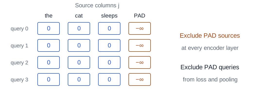
For a scored query at position \(t\), combine padding and any causal restriction before row softmax:

\[ M_{tj}=\begin{cases} 0,&m_j=1\text{ and the task permits source }j,\\ -\infty,&\text{otherwise}. \end{cases} \]

An unrestricted encoder permits all real sources; a causal stack additionally requires \(j\le t\). At least one source must remain available per computed softmax row. Empty sequences and padded query rows with no allowed source need explicit handling, rather than an all-\(-\infty\) softmax. Right padding, with at least one real token, leaves real sources available to the padded queries in this simple construction.

A source mask does not remove a padded query’s output: that query can still read real values and produce a nonzero row. Exclude such rows separately from pooling and losses. If \(v_t\) indicates a valid scored target, the token-loss mean is

\[ \mathcal L=\frac{\sum_t v_t[-\log p_{t,y_t}]}{\sum_t v_t},\qquad \sum_t v_t>0. \]

The target-validity indicator \(v_t\) need not equal input-validity \(m_t\): a final real token may have no next-token target. For a batch, sum numerator and denominator over examples and positions to obtain a mean per valid target. Averaging each sequence first and then averaging sequences gives different weighting when lengths differ. Avoid evaluating an invalid target index before selecting valid entries; setting its loss weight to zero afterward may be too late.

Mask conventions also differ between APIs. For PyTorch nn.MultiheadAttention, a Boolean mask’s True excludes an entry; check the documented convention rather than assuming every attention function uses the same rule (PyTorch 2.8 documentation).

Shift the target one position ahead

Return to the proverb. The vocabulary head now has \(C=K=9\) output classes, while the contextual feature width remains \(D=5\):

\[ \mathbf s_t=\mathbf h_{\mathrm{enc},t}W_o^\top+\mathbf b_o, \qquad W_o\in\mathbb R^{9\times5}. \]

Using the token IDs \(k_t\) defined in the token lookup, the next-token target is \(y_t=k_{t+1}\). For example:

Table 33: Next-token alignment for selected proverb positions. The target with is supplied by the training continuation, not included in the seven-token prediction prefix.

Input position	Token in the input	Token to predict	Allowed input through this position
0	a	journey	a
1	journey	of	a journey
5	miles	begins	a journey of a thousand miles
6	begins	with	a journey of a thousand miles begins

If an example contains only the seven prefix tokens and no continuation, its first six rows have next-token targets; the begins row does not. If the training record also supplies with, that value can label the final prefix row. It must not enter the inputs used for that prediction.

To train many next-token predictions from one complete record, use causal self-attention in every block. For instance, an unrestricted miles row could read the future input begins, which is exactly its target. A causal mask only in the last block cannot undo future information already mixed by an earlier unrestricted block. Row-wise normalization, the MLP, and residual paths preserve a correctly established boundary; they do not establish it on their own.

This is a causal self-attention stack for autoregressive prediction. Our worked encoder used unrestricted context over a fully supplied prefix. The same building blocks support both routes, but their visibility and training objectives differ. A complete encoder–decoder model would add a decoder and cross-attention to encoder outputs; that architecture is outside this chapter’s encoder walkthrough (Vaswani et al., §§3.1–3.2).

NotePause and predict: can the model see the answer?

You train the miles row to predict begins. The complete record contains both words. The first block uses unrestricted attention and the second uses a causal mask. Is the prediction protected from future information?

Reveal the explanation

No. The first block can mix begins into the miles representation. The second block’s causal mask cannot remove that dependence from its own input. Apply the visibility restriction at every attention layer and keep the next-token targets shifted relative to the inputs.

Teacher forcing is not the generation loop

During teacher-forced training or evaluation, each prefix contains the recorded previous tokens, and each row predicts the next recorded token. The targets provide a loss; they do not become visible future inputs to the scored row. All rows of a known record can be calculated together under a causal mask.

During generation, read the vocabulary distribution from the last supplied row, select a token using a declared rule such as argmax or sampling, append that selected token to the prefix, and predict again. Thus a hypothetical selection of with would produce an eight-token prefix for the next step. Our hand-chosen parameters do not demonstrate that selection or successful proverb completion. No EOS token was defined in the toy vocabulary, so the teaching example needs an externally chosen generation length; a system with EOS would define its ID and stopping rule explicitly.

Generated prefixes can contain mistakes that recorded prefixes do not. Therefore, next-token accuracy on teacher-forced inputs and the quality of a generated sequence answer different questions. A causal stack can parallelize positions in a known training sequence, but generating unknown future tokens remains sequential across generation steps.

What does the tutorial experiment establish?

The Week 06 tutorial uses a tiny robot-command language rather than the proverb. An episode has the form BOS cue … RECALL cue EOS. The cue is one of four movement directions; \(d\) independent random movement commands intervene before RECALL. Predicting the movement after RECALL requires remembering the initial cue. Here cue-recall accuracy means the fraction of these requests answered correctly, not the usual classification metric named recall.

Random movement targets are independent of the history. Their four-way uncertainty remains even with perfect memory: a uniform movement predictor has expected accuracy \(1/4\) and cross-entropy \(\log4\approx1.39\) nats. An all-token score mixes this uncertainty with the learnable cue dependency and deterministic episode structure, so it can conceal whether memory is working.

The stored comparison uses 4,096 training, 512 validation, and 1,024 test episodes per delay, with separate episode-generation seeds. It trains RNN, GRU, and one-block causal Transformer recipes for 60 epochs using the same episodes and batch orders, Adam at 0.003, and gradient clipping at one. Each run selects its checkpoint using validation cue-recall cross-entropy, before test scoring. Three initialization seeds, 6206/6207/6208, are retained rather than selecting a favorable test seed.

These trained recipes differ from the textbook arithmetic: their embeddings have width 16 for the recurrent models and 12 for the Transformer, their vocabulary has seven robot tokens, and the Transformer uses learned positions. RNN/GRU hidden widths are 32/17; the Transformer has two width-six heads and MLP width 24. Parameter counts are close (1,943/2,023/1,915), but that does not equalize computation or capacity.

Table 34: Held-out cue-recall accuracy (fraction correct), mean ± sample standard deviation over three initializations. Each delay uses 1,024 fixed test episodes; these spreads are not confidence intervals. Values are taken from the tutorial’s stored results and rounded to three significant digits.

Model	Delay 8	Delay 16	Delay 32
RNN	1 ± 0	0.44 ± 0.126	0.257 ± 0
GRU	1 ± 0	0.814 ± 0.116	0.322 ± 0.102
Transformer	1 ± 0	1 ± 0	1 ± 0

At delay 8, all three recipes achieve perfect cue-recall accuracy on these test episodes. At delay 16, the RNN mean is below one half, the GRU mean is about four fifths, and the Transformer succeeds for every retained initialization. At delay 32, the recurrent recipes struggle while the Transformer succeeds on this fixed-position dependency. A small seed spread can mean consistently poor results, as the delay-32 RNN shows. The spread concerns initialization on one fixed dataset; it is not a confidence interval or evidence about independently sampled datasets.

These results support this comparison under its task, budget, and checkpoint rule. They do not establish universal superiority, length extrapolation, or successful language generation. Each delay is trained separately; the initial cue position is fixed, and the trained Transformer can retrieve it directly. The tutorial retains per-seed cross-entropies, reference predictors, compute measurements, and cue interventions for a fuller interpretation. Its optional forecasting extension also distinguishes predicting one observed-data step from sustaining a rollout. Real time series may require chronological splits and separation of overlapping windows rather than randomly split episodes.

Attention’s shorter path has a computation cost

An RNN passes information between distant positions through repeated transitions; full attention can connect any allowed pair in one layer. A shorter dependency path helps information reach distant rows, but does not guarantee successful learning or make every implementation faster.

For one head, query-key matching costs on the order of \(T^2d_k\) operations and value mixing \(T^2d_v\). Explicitly materialized score and weight arrays have \(T^2\) entries per head. Tiled exact-attention implementations such as FlashAttention can avoid storing these whole arrays, although full pairwise attention still performs quadratic pair arithmetic. Projection maps and the MLP add further work; under standard head widths their typical terms scale as \(TD^2\) and \(TDF\). These are shape-based operation counts, not measured wall-clock predictions. Batch size, head count, depth, hardware, and implementation also matter (Vaswani et al., §4).

Images can supply tokens too

A Vision Transformer (ViT) replaces word lookup with patch projection. For an image of height \(H_{\mathrm{img}}\), width \(W_{\mathrm{img}}\), and \(C_{\mathrm{img}}\) channels, nonoverlapping square patches of side \(p\) give \(N_{\mathrm{patch}}=(H_{\mathrm{img}}/p)(W_{\mathrm{img}}/p)\) patches when the dimensions are divisible by \(p\). Flatten each patch into \(p^2C_{\mathrm{img}}\) numbers, then project to model width \(D\).

Figure 17: The lecture’s ViT example divides a six-by-six grayscale image into four three-by-three patches, flattens and projects each patch, prepends a class token, and adds position information before an encoder. It is a separate shape example, not our seven-word numerical model. Original course figure reused from the Week 06 lecture.

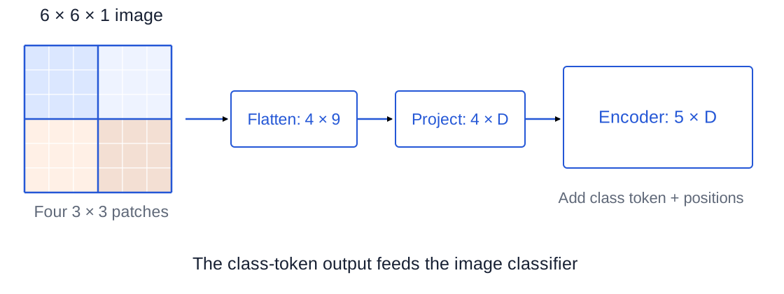
The example in Figure 17 has four patches with nine input features each; projection to \(D=4\) gives four feature rows. Adding a learned class token gives \(T=5\) rows, and position vectors identify their spatial arrangement. Encoder blocks contextualize these rows; a classifier reads the class-token output. The original ViT uses a pre-norm encoder, a final normalization, and GELU in its MLP; our small arithmetic used ReLU (Dosovitskiy et al. 2021). The mechanism connects to Week 05’s image representations, while replacing local convolutional mixing with attention over patch tokens. The choice of token construction changes the input, not the need for a task head and evaluation.

Synthesis, optional exercises, and further reading

Follow the information, then follow the learning signal

A recurrent model updates a state using one shared cell. Backpropagation follows the unrolled dependencies: local derivatives multiply along a path, and contributions from shared uses add. Long products explain why simple recurrent models can struggle to learn distant dependencies. Gates introduce controlled carry and write paths, while clipping limits large gradients without restoring vanished ones.

Attention builds a contextual row by projecting queries, keys, and values, comparing queries with permitted source keys, normalizing scores across sources, and taking weighted sums of values. Multiple heads retain several such mixtures before an output projection returns to model width. The encoder combines that operation with row-wise normalization, a shared row MLP, and two residual additions. Position information distinguishes arrangements; the task head supplies predictions; masks and target alignment enforce the information boundary.

This development also puts the methods in context. The original 2017 Transformer combined attention-based encoder and decoder stacks for sequence transduction; this chapter has concentrated on its encoder building blocks and distinguished their causal variant. Vision Transformer later used an encoder for projected image patches rather than words (Dosovitskiy et al. 2021). The common thread is learning useful intermediate representations, with the architecture specifying how information can move between their coordinates and positions.

Common confusions to resolve

Table 35: A reading checklist for sequence models and Transformer encoders.

Confusion	What to check instead
A hidden feature is already a prediction.	Identify the task head, target, and loss.
A longer RNN has a new cell’s parameters at every step.	One shared parameter receives gradient contributions from all its uses.
A nonzero shared-weight gradient proves long-range learning.	Later uses may supply the gradient while early paths have vanished.
Seven attention weights mean seven output features.	Weights index source positions; the weighted values determine feature width.
Attention softmax predicts the next word.	It normalizes source scores; a vocabulary head normalizes class logits.
Heads split the sentence into chunks.	Each head projects the full input and uses its own permitted source mixture.
LayerNorm mixes words or uses batch running statistics.	Here its statistics come from the features of one current row.
The second bypass returns to the original input.	It carries U, the representation after the first addition.
Masking padding sources is enough.	Also exclude padded outputs from pooling and invalid targets from loss.
A last-layer causal mask prevents all future leakage.	Check visibility at every earlier attention layer too.
Parallel training means parallel generation of unknown tokens.	A known record and a generated prefix provide different inputs.
A toy task establishes an architecture ranking for all data.	Read the task, split, budget, selection rule, and evaluation protocol.

Optional exercises

These exercises ask for reasoning beyond the worked examples; answers are not included here.

1. Change the readout location. In the zero-bias three-step scalar RNN, replace the final-only objective by \(\mathcal L=\tfrac12(\widehat y_1-y_1)^2+\tfrac12(\widehat y_2-y_2)^2\), with \(\widehat y_t=w_oh_t\). Derive the two direct head contributions and the resulting \(g_1^h\). Explain how the shared \(w_o\) gradient changes.
2. Separate state bounds from gradient bounds. For an identity-activation scalar RNN with \(w_h=-0.8\), calculate \(\partial h_{s+5}/\partial h_s\), the factor that carries sensitivity backward across five transitions. What are its sign and magnitude? Then explain why bounded tanh states do not alone determine the gradient magnitude.
3. Inspect a mask before computing. One query has three scores \((0,\log2,\log3)\) and scalar values \((2,-1,4)\). Compute its unrestricted output. Label the sources \(j=0,1,2\). Then exclude source \(j=2\) (the third source), renormalize, and compute the masked output. Explain why simply replacing its already-normalized weight with zero gives a different result.
4. Change the head count. Use three heads with \(d_k=2\), \(d_v=4\), input width \(D=5\), and seven positions. Give shapes for Q/K/V, each score matrix, the concatenation, the stored output projection, and its right multiplier. Is this the standard equal-partition configuration of nn.MultiheadAttention?
5. Find the two bypasses. Write a pre-norm block’s output when its attention branch is identically zero. Then set its MLP branch to zero too. Does a separate final LayerNorm necessarily return the unchanged original representation? State the distinction between a block and the stack.
6. Audit an evaluation. A report selects the seed with best test cue-recall accuracy and pools padded query rows into a sequence vector. Identify the two problems and propose separate repairs. State what additional evaluation would be needed to claim generalization to delays never used for training.

Further reading and executable companions

• Goodfellow, Bengio, and Courville, Deep Learning, Chapter 10: recurrent computation and learning over sequences.
• Pascanu, Mikolov, and Bengio (2013): recurrent gradient difficulty and clipping.
• Vaswani et al., Attention Is All You Need: the original encoder–decoder Transformer, scaled attention, multiple heads, and positional encoding. Its post-norm layout differs from our main pre-norm walkthrough.
• Xiong et al., On Layer Normalization in the Transformer Architecture: why normalization placement matters for optimization.
• Dosovitskiy et al., An Image Is Worth 16x16 Words: the image-patch encoder connection.
• Week 06 tutorial: executable recurrent/attention calculations, robot-cue interventions, held-out comparison, and optional forecasting diagnostics.

The chapter’s small ledgers establish how the operations compose. The tutorial’s experiments ask whether a trained recipe uses the information that a task requires. Keep those two forms of evidence distinct when reading a model description or designing a comparison.

Dosovitskiy, Alexey, Lucas Beyer, Alexander Kolesnikov, et al. 2021. “An Image Is Worth 16x16 Words: Transformers for Image Recognition at Scale.” International Conference on Learning Representations. https://arxiv.org/abs/2010.11929.

Goodfellow, Ian, Yoshua Bengio, and Aaron Courville. 2016. Deep Learning. MIT Press. https://www.deeplearningbook.org/.