Sequential
representation
learning

Week-06 · ML-2026

RNNs and Transformer encoders

Alexei Kornaev,
Dr. Sc., Prof.

Innopolis University

Researcher at the RC for AI,
National RC for Oncology n.a. N.N. Blokhin

Instructor-supplied graphical abstract with the handwritten phrase All you need is… on a white background.

Lecture map

  1. Sequence problems and recurrent state
  2. Learning through time and gated memory
  3. Self-attention and contextual representations
  4. Inside a Transformer encoder

Print / save as PDF

Session 1: Parts 1–2. Session 2: Parts 3–4.
Code inspection remains a separate, flexible part of each session.

What should you be able to explain?

  • Trace a recurrent state forward and shared-parameter gradients backward
  • Calculate query–key scores and a weighted value mixture
  • Reconstruct an encoder block and choose visibility for its task

Track positions, feature widths, parameter sharing, and permitted inputs.

Notation: positions and representations

Symbol Meaning
t=0,…,T−1t=0,\ldots,T-1 Position within one sequence
xt∈ℝDx_t\in\mathbb R^D Input row vector at position tt
zt,ht∈ℝHz_t,h_t\in\mathbb R^H Preactivation and recurrent state
h(ℓ)∈ℝT×Dh^{(\ell)}\in\mathbb R^{T\times D} All token representations at encoder layer ℓ\ell
θ,ℒ\theta,\ \mathcal L Trainable parameters and the stated loss

Subscripts locate a position. Superscripts locate a layer.

Part 1 · Sequence problems and recurrent state

  1. Sequence problems and recurrent state
  2. Learning through time and gated memory
  3. Self-attention and contextual representations
  4. Inside a Transformer encoder

How can the current prediction use earlier observations?

Sequences contain ordered observations

Four measurements, four words, and four image patches each form an ordered sequence. Position refers to the supplied order, not necessarily physical time. Measurementsx₀x₁x₂x₃WordsthedogbitesSamImage patchespatch 0patch 1patch 2patch 3Position indexes the order supplied to the model

The position axis adds structure to the feature axis.

The task determines where outputs belong

Task Observed input Output Example
Sequence classification x0,…,xT−1x_0,\ldots,x_{T-1} One label Classify an utterance
Position-wise labeling x0,…,xT−1x_0,\ldots,x_{T-1} One label per position Label each word’s role
Next-observation prediction x0,…,xtx_0,\ldots,x_t Predict position t+1t+1 Forecast a measurement

Specify the information available at the moment of prediction.

Student question 1 · Does order change the answer?

Sequences minus one, zero, one and one, zero, minus one have equal means but opposite trends. Rising-101012Position tFalling-101012Position t

Task: classify the direction of the trend. Can the mean distinguish these sequences?

Both means are 00. Their ordered changes have opposite signs.

A fixed window is already a valid input

xflat=[x0∣x1∣⋯∣xT−1]∈ℝTDx_{\mathrm{flat}}=[x_0\mid x_1\mid\cdots\mid x_{T-1}]\in\mathbb R^{TD}

ŷ=f(xflat;θ)\widehat y=f(x_{\mathrm{flat}};\theta)

An MLP can use order

Each window position occupies distinct input coordinates.

Its input width is fixed

A new window length needs an explicit handling rule.

An RNN offers a shared update for successive positions.

A recurrent state carries the earlier computation

A current input and the previous state enter a shared affine-and-tanh recurrent cell to produce the new state. A recurrent cell updates a stateprevious stateaffine + tanhnew statecurrent inputParameters define the update; the state changes with the observations

ht=fcell(xt,ht−1;θ)h_t=f_{\mathrm{cell}}(x_t,h_{t-1};\theta)

The state changes at each position. The cell parameters are shared.

One recurrent unit combines input and memory

Two input coordinates, two state coordinates. Here j∈{1,2}j\in\{1,2\}.

One tanh unit combines both current input coordinates, both previous state coordinates, and a bias to produce one new hidden coordinate. Current inputPrevious statexₜ,₁xₜ,₂hₜ₋₁,₁hₜ₋₁,₂Σtanhhₜ,ⱼWₓWₕbₕ,ⱼzₜ,ⱼOne unit j of a two-unit state

1 · Current input It,j=∑k=12Wx,jkxt,kI_{t,j}=\sum_{k=1}^{2}W_{x,jk}x_{t,k}

2 · Previous state Rt,j=∑r=12Wh,jrht−1,rR_{t,j}=\sum_{r=1}^{2}W_{h,jr}h_{t-1,r}

3 · Affine sum zt,j=It,j+Rt,j+bh,jz_{t,j}=I_{t,j}+R_{t,j}+b_{h,j}

4 · Activation ht,j=tanh⁡(zt,j)h_{t,j}=\tanh(z_{t,j})

Every state coordinate has its own weights and bias.

RNN formulation: Goodfellow, Bengio & Courville, Chapter 10. Original course diagram.

Two ordinary units form one recurrent state

zt=xtWx⊤+ht−1Wh⊤+bhz_t=x_tW_x^\top+h_{t-1}W_h^\top+b_h

ht=tanh⁡(zt)h_t=\tanh(z_t)

Quantity Shape Role
xtx_t, ht−1h_{t-1} DD, HH Current features, previous state
WxW_x, WhW_h H×DH\times D, H×HH\times H One row per state unit
bhb_h, ztz_t, hth_t HH Bias, affine sum, activation

The same row-vector convention extends Week 04’s affine layer.

Small numbers make the forward pass visible

Three observations from two numerical features. Illustrative, untrained parameters.

Wx=[0.3−0.20.10.4]W_x=\begin{bmatrix}0.3&-0.2\\0.1&0.4\end{bmatrix} Wh=[0.50.1−0.20.3]W_h=\begin{bmatrix}0.5&0.1\\-0.2&0.3\end{bmatrix} bh=(0.05,−0.10),h−1=(0,0)b_h=(0.05,-0.10),\quad h_{-1}=(0,0)

Position Input xtx_t
00 (1.0,−0.5)(1.0,-0.5)
11 (0.2,0.8)(0.2,0.8)
22 (−0.4,0.3)(-0.4,0.3)

Both input coordinates may be signed, as with standardized sensor features.

All three steps reuse these same ten cell parameters.

The first observation creates a state

x0=(1.0,−0.5)x_0=(1.0,-0.5) and h−1=(0,0)h_{-1}=(0,0).

1 · Current-input contribution x0Wx⊤=(0.4000,−0.1000)x_0W_x^\top=(0.4000,-0.1000)

2 · Previous-state contribution h−1Wh⊤=(0,0)h_{-1}W_h^\top=(0,0)

3 · Add the bias z0=(0.4000,−0.1000)+(0.05,−0.10)=(0.4500,−0.2000)z_0=(0.4000,-0.1000)+(0.05,-0.10)=(0.4500,-0.2000)

4 · Apply tanh to each coordinate h0=(0.4219,−0.1974)h_0=(0.4219,-0.1974)

A zero initial state leaves the input and bias paths active.

The next observation combines with the earlier state

x1=(0.2,0.8)x_1=(0.2,0.8) and the computed h0=(0.4219,−0.1974)h_0=(0.4219,-0.1974).

1 · Current-input contribution x1Wx⊤=(−0.1000,0.3400)x_1W_x^\top=(-0.1000,0.3400)

2 · Previous-state contribution h0Wh⊤=(0.1912,−0.1436)h_0W_h^\top=(0.1912,-0.1436)

3 · Add both contributions and the bias z1=(−0.1000,0.3400)+(0.1912,−0.1436)+(0.05,−0.10)z_1=(-0.1000,0.3400)+(0.1912,-0.1436)+(0.05,-0.10) z1=(0.1412,0.0964)z_1=(0.1412,0.0964)

4 · Apply tanh h1=(0.1403,0.0961)h_1=(0.1403,0.0961)

Unrolling makes the dependency graph visible

Three observations enter three uses of the same recurrent cell. Hidden states carry information from left to right; the initial state is zero. Same Wₓ, Wₕ, bₕ at every positionh₋₁ = 0h₀x₀h₁x₁h₂x₂
tt xtx_t ztz_t hth_t
0 (1.0000,−0.5000)(1.0000, -0.5000) (0.4500,−0.2000)(0.4500, -0.2000) (0.4219,−0.1974)(0.4219, -0.1974)
1 (0.2000,0.8000)(0.2000, 0.8000) (0.1412,0.0964)(0.1412, 0.0964) (0.1403,0.0961)(0.1403, 0.0961)
2 (−0.4000,0.3000)(-0.4000, 0.3000) (−0.0502,−0.0192)(-0.0502, -0.0192) (−0.0502,−0.0192)(-0.0502, -0.0192)

Each state depends on a prefix through repeated uses of one cell.

Student question 2 · Do longer sequences add parameters?

Our cell has D=H=2D=H=2.

Wx:2×2,Wh:2×2,bh:2W_x:\ 2\times2,\qquad W_h:\ 2\times2,\qquad b_h:\ 2

If we process six positions instead of three, how many trainable cell parameters do we use?

Still 4+4+2=104+4+2=10. There are more computations and saved states.

An output head gives the state a task

at=htWo⊤+bo∈ℝCa_t=h_tW_o^\top+b_o\in\mathbb R^C

pt=softmax⁡(at)p_t=\operatorname{softmax}(a_t)

Classification

CC logits support a distribution over CC classes.

Regression

An affine head can predict a continuous target directly.

Hidden coordinates, logits, and probabilities have different roles.

Part 2 · Learning through time and gated memory

  1. Sequence problems and recurrent state
  2. Learning through time and gated memory
  3. Self-attention and contextual representations
  4. Inside a Transformer encoder

A shared parameter receives a contribution from every use.

A final-state loss starts a simple backward pass

First microscope: identity readout, target y=(0.20,−0.15)y=(0.20,-0.15).

ℒ=12∥h2−y∥22\mathcal L=\frac12\|h_2-y\|_2^2

h2=(−0.0502,−0.0192),ℒ≈0.039853h_2=(-0.0502,-0.0192),\qquad \mathcal L\approx0.039853

g2h=∂ℒ∂h2=h2−y=(−0.2502,0.1308)g^h_2=\frac{\partial\mathcal L}{\partial h_2}=h_2-y=(-0.2502,0.1308)

A loss derivative describes sensitivity, not a parameter update.

The activation supplies a local derivative

ht,j=tanh⁡(zt,j)h_{t,j}=\tanh(z_{t,j})

∂ht,j∂zt,j=1−ht,j2\frac{\partial h_{t,j}}{\partial z_{t,j}}=1-h_{t,j}^2

gtz=gth⊙(1−ht2)g^z_t=g^h_t\odot(1-h_t^2)

At t=2t=2: (1−h22)=(0.9975,0.9996)(1-h_2^2)=(0.9975,0.9996),

g2z=(−0.2496,0.1307).g^z_2=(-0.2496,0.1307).

One final loss travels backward through time

Three steps, h−1=0h_{-1}=0. Here ℒ=12∥h2−y∥2\mathcal L=\tfrac12\|h_2-y\|^2 for a target vector yy.

Three recurrent states share parameters. A final-state loss sends gradients backward through the unrolled recurrence. One cell, three uses of the same parametersh₀x₀h₁x₁h₂x₂h₋₁ℒloss signalbackward through Wₕ

1 · Loss and final activation g2h=h2−y,g2z=g2h⊙(1−h22)g^h_2=h_2-y,\quad g^z_2=g^h_2\odot(1-h_2^2)

2 · Previous state receives a signal gth=gt+1zWh,t=1,0g^h_t=g^z_{t+1}W_h,\quad t=1,0

3 · Repeat the local chain rule gtz=gth⊙(1−ht2),t=1,0g^z_t=g^h_t\odot(1-h_t^2),\quad t=1,0

4 · Sum contributions to one shared matrix ∂ℒ∂Wh=∑t=02(gtz)⊤ht−1\frac{\partial\mathcal L}{\partial W_h}=\sum_{t=0}^{2}(g^z_t)^\top h_{t-1}

gth=∂ℒ/∂htg^h_t=\partial\mathcal L/\partial h_t and gtz=∂ℒ/∂ztg^z_t=\partial\mathcal L/\partial z_t are row vectors.

Chain rule and parameter sharing: Goodfellow, Bengio & Courville, Chapter 10. ⊙\odot and the square act coordinate-wise.

The same chain rule reaches earlier states

Backward order gthg^h_t 1−ht21-h_t^2 gtzg^z_t
t=2t=2 (−0.2502,0.1308)(-0.2502, 0.1308) (0.9975,0.9996)(0.9975, 0.9996) (−0.2496,0.1307)(-0.2496, 0.1307)
t=1t=1 (−0.1509,0.0143)(-0.1509, 0.0143) (0.9803,0.9908)(0.9803, 0.9908) (−0.1480,0.0141)(-0.1480, 0.0141)
t=0t=0 (−0.0768,−0.0106)(-0.0768, -0.0106) (0.8220,0.9610)(0.8220, 0.9610) (−0.0631,−0.0101)(-0.0631, -0.0101)

gt−1h=gtzWh,gt−1z=gt−1h⊙(1−ht−12)g^h_{t-1}=g^z_tW_h,\qquad g^z_{t-1}=g^h_{t-1}\odot(1-h_{t-1}^2)

Read the ledger from the final position back to the first.

One weight use contributes an outer product

zt,j=∑kWx,jkxt,k+∑rWh,jrht−1,r+bh,jz_{t,j}=\sum_k W_{x,jk}x_{t,k}+\sum_r W_{h,jr}h_{t-1,r}+b_{h,j}

∂ℒ∂Wh,jr|use at t=gt,jzht−1,r\left.\frac{\partial\mathcal L}{\partial W_{h,jr}}\right|_{\text{use at }t}=g^z_{t,j}h_{t-1,r}

Gt=(gtz)⊤ht−1∈ℝH×HG_t=(g^z_t)^\top h_{t-1}\in\mathbb R^{H\times H}

Rows index receiving units. Columns index previous-state coordinates.

Shared weights receive the sum of their uses

Use at t = 0

[0.00000.00000.00000.0000]\begin{bmatrix}0.0000 & 0.0000\\0.0000 & 0.0000\end{bmatrix}

Use at t = 1

[−0.06240.02920.0060−0.0028]\begin{bmatrix}-0.0624 & 0.0292\\0.0060 & -0.0028\end{bmatrix}

Use at t = 2

[−0.0350−0.02400.01830.0126]\begin{bmatrix}-0.0350 & -0.0240\\0.0183 & 0.0126\end{bmatrix}

Sum

[−0.09740.00520.02430.0098]\begin{bmatrix}-0.0974 & 0.0052\\0.0243 & 0.0098\end{bmatrix}

∂ℒ∂Wh=G0+G1+G2\frac{\partial\mathcal L}{\partial W_h}=G_0+G_1+G_2

The contributions add to one matrix. They may reinforce or cancel.

Student question 3 · Which shared-weight uses matter?

Only the final state has a loss. The matrix WhW_h appears at t=0,1,2t=0,1,2.

Should its gradient include just the last use, or all three uses?

Sum all uses. In this example, the t=0t=0 term is zero because h−1=0h_{-1}=0.

A loss at every position adds direct signals

Second microscope: C=3C=3 classes, target IDs (y0,y1,y2)=(0,2,1)(y_0,y_1,y_2)=(0,2,1).

at=htWo⊤+bo,pt=softmax⁡(at)a_t=h_tW_o^\top+b_o,\quad p_t=\operatorname{softmax}(a_t)

ℓt=−log⁡pt[yt],ℒ=1T∑t=0T−1ℓt\ell_t=-\log p_t[y_t],\qquad \mathcal L=\frac1T\sum_{t=0}^{T-1}\ell_t

gta=pt−onehot⁡(yt)Tg^a_t=\frac{p_t-\operatorname{onehot}(y_t)}{T}

For this mean objective, divide by TT once at the loss derivative.

The same states produce three-class predictions

Wo=[0.4−0.2−0.30.50.10.2]W_o=\begin{bmatrix}0.4&-0.2\\-0.3&0.5\\0.1&0.2\end{bmatrix} bo=(0.02,−0.04,0.01)b_o=(0.02,-0.04,0.01)

At the final position:

p2=(0.3379,0.3252,0.3370)p_2=(0.3379,0.3252,0.3370)

Target ID: y2=1y_2=1.

Mean loss across all three positions:

ℒ≈1.027996nats\mathcal L\approx1.027996\ \text{nats}

The output head changes the objective and its direct gradient paths.

A hidden state receives direct and future gradients

1 · Direct signal through this position’s output head gt,directh=gtaWog^h_{t,\text{direct}}=g^a_tW_o

2 · Add the signal from the next recurrent use gth=gtaWo+gt+1zWhg^h_t=g^a_tW_o+g^z_{t+1}W_h

3 · Pass through the local activation gtz=gth⊙(1−ht2)g^z_t=g^h_t\odot(1-h_t^2)

At the final position, the future contribution is zero.

Goodfellow, Bengio & Courville (2016), Chapter 10. Derivatives independently checked.

The recurrent parameters collect local contributions

∂ℒ∂Wx=∑t(gtz)⊤xt\frac{\partial\mathcal L}{\partial W_x}=\sum_t(g^z_t)^\top x_t

∂ℒ∂Wh=∑t(gtz)⊤ht−1\frac{\partial\mathcal L}{\partial W_h}=\sum_t(g^z_t)^\top h_{t-1}

∂ℒ∂bh=∑tgtz\frac{\partial\mathcal L}{\partial b_h}=\sum_t g^z_t

The local input changes by position. The parameter is shared.

The output head also shares its parameters

∂ℒ∂Wo=∑t(gta)⊤ht\frac{\partial\mathcal L}{\partial W_o}=\sum_t(g^a_t)^\top h_t

∂ℒ∂bo=∑tgta\frac{\partial\mathcal L}{\partial b_o}=\sum_t g^a_t

θ←θ−η∇θℒ\theta\leftarrow\theta-\eta\nabla_\theta\mathcal L

Compute the complete gradient before the optimizer changes parameters.

Two independent checks support the derivation

Objective Checked parameters Max. finite-difference error Max. autograd error
Final-state squared error 10 scalars 3.19×10−123.19\times10^{-12} 5.55×10−175.55\times10^{-17}
Mean three-position CE 19 scalars 1.71×10−101.71\times10^{-10} 6.94×10−176.94\times10^{-17}

∂ℒ∂θj≈ℒ(θj+ϵ)−ℒ(θj−ϵ)2ϵ,ϵ=10−6\frac{\partial\mathcal L}{\partial\theta_j}\approx\frac{\mathcal L(\theta_j+\epsilon)-\mathcal L(\theta_j-\epsilon)}{2\epsilon},\quad \epsilon=10^{-6}

Finite differences and PyTorch autograd agree with manual BPTT.

Original float64 calculations. Full numerical ledger.

Long paths multiply local Jacobians

Dt=diag⁡(1−ht2)D_t=\operatorname{diag}(1-h_t^2)

gt−1h=gthDtWhg^h_{t-1}=g^h_tD_tW_h

gsh=gth(DtWh)(Dt−1Wh)⋯(Ds+1Wh)g^h_s=g^h_t(D_tW_h)(D_{t-1}W_h)\cdots(D_{s+1}W_h)

Along one future-loss path, every transition changes the sensitivity.

Repeated factors can shrink or amplify a signal

For a toy scalar constant local derivative, sensitivities 0.7 to the power n decay, 1 stays constant, and 1.2 to the power n grows over zero to 32 transitions. This is not a trained RNN measurement. Repeated multiplication changes gradient reach10^-510^-310^-110^110^308162432r = 0.7r = 1.0r = 1.2Number of transitions nVertical axis: sensitivity magnitude on a log₁₀ scale

Toy scalar case: a constant local derivative rr gives |r|n|r|^n.

Original illustrative calculation; Pascanu et al. (2013) analyzes the matrix case.

Gradient clipping limits a large update direction

g=∇θℒ,c>0g=\nabla_\theta\mathcal L,\qquad c>0

g̃={g,∥g∥2≤c,c∥g∥2g,∥g∥2>c.\widetilde g=\begin{cases}g,&\|g\|_2\le c,\\\displaystyle\frac{c}{\|g\|_2}g,&\|g\|_2>c.\end{cases}

∥g̃∥2≤c\|\widetilde g\|_2\le c

Clipping caps large gradients. It cannot recover a vanished signal.

A GRU learns how much old state to retain

One illustrative GRU coordinate retains 0.9 times the old state 0.5 and writes 0.1 times the candidate minus 0.4, giving 0.41. One state coordinateold state 0.5candidate −0.4retain × 0.9write × 0.1+new state 0.41

ht=ut⊙ht−1+(1−ut)⊙h̃th_t=u_t\odot h_{t-1}+(1-u_t)\odot\widetilde h_t

A gate near one retains that coordinate. A gate near zero favors the candidate.

PyTorch GRU equations. Here utu_t names its update gate ztz_t.

GRU gates depend on the input and previous state

ut,rt,h̃t,ht∈ℝHu_t,r_t,\widetilde h_t,h_t\in\mathbb R^H. σ\sigma is the logistic sigmoid.

Retention/update gate ut=σ(xtWxu⊤+bxu+ht−1Whu⊤+bhu)u_t=\sigma(x_tW_{xu}^\top+b_{xu}+h_{t-1}W_{hu}^\top+b_{hu})

Reset gate rt=σ(xtWxr⊤+bxr+ht−1Whr⊤+bhr)r_t=\sigma(x_tW_{xr}^\top+b_{xr}+h_{t-1}W_{hr}^\top+b_{hr})

Candidate state h̃t=tanh⁡(xtWxn⊤+bxn+rt⊙(ht−1Whn⊤+bhn))\widetilde h_t=\tanh\!\left(x_tW_{xn}^\top+b_{xn}+r_t\odot(h_{t-1}W_{hn}^\top+b_{hn})\right)

Retention controls the mixture. Reset controls recurrent input to the candidate.

PyTorch GRU: reset after the recurrent affine operation.

An LSTM separates cell storage from its visible state

An LSTM cell retains f times the old cell state and adds i times a candidate. A separate output gate reads tanh of the updated cell state into the hidden state. Cell state and visible state have separate pathscₜ₋₁× fₜ+cₜcandidate× iₜtanh× oₜhₜRetainWriteRead

ct=ft⊙ct−1+it⊙c̃tc_t=f_t\odot c_{t-1}+i_t\odot\widetilde c_t ht=ot⊙tanh⁡(ct)h_t=o_t\odot\tanh(c_t)

Forget, input, and output gates control retention, writing, and reading.

PyTorch LSTM equations. Plain LSTM, without projection or peephole connections.

Part 3 · Self-attention and contextual representations

  1. Sequence problems and recurrent state
  2. Learning through time and gated memory
  3. Self-attention and contextual representations
  4. Inside a Transformer encoder

Each position forms a weighted combination of permitted source representations.

The same token can need different context

The word bank appears near river in one phrase and loan in another, motivating contextual representations without claiming trained attention scores. theriverbankthebankloanThe same token can need different contextual representations

A contextual representation depends on the surrounding sequence.

Token lookup supplies an initial representation

stis a token ID,et=E[st]∈ℝDs_t\ \text{is a token ID},\qquad e_t=E[s_t]\in\mathbb R^D

ht(0)=et+ptposh_t^{(0)}=e_t+p_t^{\mathrm{pos}}

Token information

A learned table EE maps categories to vectors.

Position information

ptposp_t^{\mathrm{pos}} identifies where a token occurs.

Token IDs are labels; their numerical magnitude has no semantic meaning.

A query matches keys and combines values

A query and candidate keys form dot-product scores. Scaling and row softmax produce weights, which combine separate source value vectors. query qₜkeys kⱼdot productsscalerow softmaxvalues vⱼweighted sumQuery–key scores choose weights; values supply the combined content

The query row chooses weights over source value rows.

One input has three learned projection maps

X∈ℝT×DX\in\mathbb R^{T\times D}

Qatt=XWQ⊤,Katt=XWK⊤Q_{\mathrm{att}}=XW_Q^\top,\quad K_{\mathrm{att}}=XW_K^\top

Vatt=XWV⊤V_{\mathrm{att}}=XW_V^\top

Weights Shape Projected rows
WQ,WKW_Q,W_K dk×Dd_k\times D Queries and keys: T×dkT\times d_k
WVW_V dv×Dd_v\times D Values: T×dvT\times d_v

Matching needs equal query/key widths. Value width may differ.

A three-token microscope fixes every input number

Positions 0,1,20,1,2: “the”, “cat”, “sleeps”. T=3T=3, D=4D=4, dk=dv=2d_k=d_v=2.

X=[101001011100]X=\begin{bmatrix}1&0&1&0\\0&1&0&1\\1&1&0&0\end{bmatrix}

Query weights

WQ=[10000100]W_Q=\begin{bmatrix}1&0&0&0\\0&1&0&0\end{bmatrix}

Key weights

WK=[00100001]W_K=\begin{bmatrix}0&0&1&0\\0&0&0&1\end{bmatrix}

Value weights

WV=[10100102]W_V=\begin{bmatrix}1&0&1&0\\0&1&0&2\end{bmatrix}

These illustrative parameters expose arithmetic, not learned language semantics.

Queries, keys, and values keep different information

QattQ_{\mathrm{att}}

[1.00000.00000.00001.00001.00001.0000]\begin{bmatrix}1.0000 & 0.0000\\0.0000 & 1.0000\\1.0000 & 1.0000\end{bmatrix}

KattK_{\mathrm{att}}

[1.00000.00000.00001.00000.00000.0000]\begin{bmatrix}1.0000 & 0.0000\\0.0000 & 1.0000\\0.0000 & 0.0000\end{bmatrix}

VattV_{\mathrm{att}}

[2.00000.00000.00003.00001.00001.0000]\begin{bmatrix}2.0000 & 0.0000\\0.0000 & 3.0000\\1.0000 & 1.0000\end{bmatrix}

q1=(0,1),k1=(0,1),v1=(0,3)q_1=(0,1),\qquad k_1=(0,1),\qquad v_1=(0,3)

The same input row produces three vectors with different roles.

One query scores all permitted source keys

Update position t=1t=1: q1=(0,1)q_1=(0,1). Source index j=0,1,2j=0,1,2.

Raw dot-product scores q1Katt⊤=(0,1,0)q_1K_{\mathrm{att}}^\top=(0,1,0)

Scale by the square root of query/key width S1,:=(0,1,0)2≈(0,0.7071,0)S_{1,:}=\frac{(0,1,0)}{\sqrt2}\approx(0,0.7071,0)

Rows locate queries; columns locate sources Stj=qtkj⊤dkS_{tj}=\frac{q_tk_j^\top}{\sqrt{d_k}}

A score measures query–key compatibility before normalization.

Scaling controls a dot product’s width dependence

qk⊤=∑r=1dkqrkrqk^\top=\sum_{r=1}^{d_k}q_rk_r

Var⁡(qk⊤)=dk\operatorname{Var}(qk^\top)=d_k

Var⁡(qk⊤dk)=1\operatorname{Var}\!\left(\frac{qk^\top}{\sqrt{d_k}}\right)=1

Toy assumptions: all query/key coordinates are independent, with mean 00 and variance 11.

Scaling counters larger score variance as the head width grows.

Row softmax turns the scores into mixing weights

A1j=exp⁡(S1j)∑m=02exp⁡(S1m)A_{1j}=\frac{\exp(S_{1j})}{\sum_{m=0}^{2}\exp(S_{1m})}

exp⁡(S1,:)≈(1,2.0281,1)\exp(S_{1,:})\approx(1,2.0281,1)

A1,:≈(0.2483,0.5035,0.2483)A_{1,:}\approx(0.2483,0.5035,0.2483)

Weights are nonnegative and sum to one within a query row.

The weights combine values, not keys

Source values v0=(2,0),v1=(0,3),v2=(1,1)v_0=(2,0),\quad v_1=(0,3),\quad v_2=(1,1)

Weighted combination O1≈0.2483(2,0)+0.5035(0,3)+0.2483(1,1)O_1\approx0.2483(2,0)+0.5035(0,3)+0.2483(1,1)

One contextual output row O1≈(0.7448,1.7587)O_1\approx(0.7448,1.7587)

The output is a feature vector; its coordinates need not sum to one.

Matrix attention performs the same calculation for every query

S=QattKatt⊤dk,A=softmax⁡rows(S),O=AVattS=\frac{Q_{\mathrm{att}}K_{\mathrm{att}}^\top}{\sqrt{d_k}},\quad A=\operatorname{softmax}_{\mathrm{rows}}(S),\quad O=AV_{\mathrm{att}}

Weights A

[0.50350.24830.24830.24830.50350.24830.40110.40110.1978]\begin{bmatrix}0.5035 & 0.2483 & 0.2483\\0.2483 & 0.5035 & 0.2483\\0.4011 & 0.4011 & 0.1978\end{bmatrix}

Outputs O

[1.25520.99300.74481.75871.00001.4011]\begin{bmatrix}1.2552 & 0.9930\\0.7448 & 1.7587\\1.0000 & 1.4011\end{bmatrix}

A:T×TA:T\times T mixes positions. O:T×dvO:T\times d_v contains output features.

Original checked arithmetic. Full numeric ledger.

Student question 4 · Which axis sums to one?

AA has shape T×TT\times T: rows are queries, columns are source positions.

Which axis sums to one, and which vectors form OtO_t?

Each query row sums to one across sources. OtO_t combines the source value vectors.

A causal mask changes which sources are available

Mtj={0,j≤t,−∞,j>t,A=softmax⁡rows(S+M)M_{tj}=\begin{cases}0,&j\le t,\\-\infty,&j>t,\end{cases}\qquad A=\operatorname{softmax}_{\mathrm{rows}}(S+M)

A1,:causal≈(0.3302,0.6698,0.0000)A^{\mathrm{causal}}_{1,:}\approx(0.3302, 0.6698, 0.0000)

O1causal≈(0.6605,2.0093)O^{\mathrm{causal}}_1\approx(0.6605, 2.0093)

Position 1 can use sources 0 and 1, while source 2 receives zero weight.

Multiple heads use separate projection parameters

One three-by-four input enters two heads with distinct projection parameters. Two three-by-two outputs concatenate to three-by-four, then an output projection mixes features while preserving width four. Each head has its own projection parametersXHead 1Head 2ConcatenateOutput projection3 × 23 × 23 × 43 × 4

O[i]=Attention⁡(XWQ,i⊤,XWK,i⊤,XWV,i⊤)O^{[i]}=\operatorname{Attention}(XW_{Q,i}^\top,XW_{K,i}^\top,XW_{V,i}^\top)

Each head can form a different combination of source features.

Concatenation collects features within each query

Query position Head 1 output Head 2 output
0 (1.2552,0.9930)(1.2552, 0.9930) (1.0000,0.6044)(1.0000, 0.6044)
1 (0.7448,1.7587)(0.7448, 1.7587) (1.0000,0.1978)(1.0000, 0.1978)
2 (1.0000,1.4011)(1.0000, 1.4011) (1.0000,0.3333)(1.0000, 0.3333)

[O[1]∣O[2]]∈ℝT×(Nheadsdv)[O^{[1]}\mid O^{[2]}]\in\mathbb R^{T\times(N_{\mathrm{heads}}d_v)}

[O[1]∣O[2]]t=1≈(0.7448,1.7587,1.0000,0.1978)[O^{[1]}\mid O^{[2]}]_{t=1}\approx(0.7448, 1.7587, 1.0000, 0.1978)

Two width-2 outputs concatenate to width 4 at every query position.

The output projection mixes head features

WO=[100.500100.50.501000.501]W_O=\begin{bmatrix}1&0&0.5&0\\0&1&0&0.5\\0.5&0&1&0\\0&0.5&0&1\end{bmatrix}

MHA⁡(X)=[O[1]∣O[2]]WO⊤\operatorname{MHA}(X)=[O^{[1]}\mid O^{[2]}]W_O^\top

MHA⁡(X)t=1≈(1.2448,1.8576,1.3724,1.0771)\operatorname{MHA}(X)_{t=1}\approx(1.2448, 1.8576, 1.3724, 1.0771)

The projection mixes features within a row and returns width D=4D=4.

Part 4 · Inside a Transformer encoder

  1. Sequence problems and recurrent state
  2. Learning through time and gated memory
  3. Self-attention and contextual representations
  4. Inside a Transformer encoder

Track the representation through one block, then through the stack.

One encoder block has two residual branches

Pre-norm encoder: first LayerNorm, attention and projection, residual addition, second LayerNorm, position-wise MLP, and second residual addition. Both bypasses carry unnormalized branch inputs. h input: T × DLN₁Attention + projectionLN₂Position-wise MLP+U+h nextT × D throughout

Pre-norm teaching variant

Attention branch U=h(ℓ)+MHA⁡(LN⁡1(h(ℓ)))U=h^{(\ell)}+\operatorname{MHA}(\operatorname{LN}_1(h^{(\ell)}))

MLP branch h(ℓ+1)=U+MLP⁡(LN⁡2(U))h^{(\ell+1)}=U+\operatorname{MLP}(\operatorname{LN}_2(U))

Input, both additions, and output: T×DT\times D.

Each branch computes a change and adds it to its own input.

Pre/post-norm distinction: Xiong et al. (2020).

Attention, LayerNorm, and MLP act on different axes

Three feature matrices distinguish attention across source positions, LayerNorm across the features of one row, and an MLP independently applied with shared weights to every row. Attention: combine positionsLayerNorm: normalize a rowMean and variance over DMLP: transform a rowφφφSame weights at each position
Operation What interacts? Parameters across positions
Attention Permitted source rows Shared projection maps
LayerNorm Features within one row Shared scale and shift
MLP Features within one row Shared affine maps

Only attention introduces new interactions between positions inside this block.

A complete block microscope

Three positions, D=4D=4, one head with dk=dv=2d_k=d_v=2. Fixed, untrained values.

h(ℓ)=[1.00000.0000−1.00002.00000.00002.00001.0000−1.00002.00001.00000.00001.0000]h^{(\ell)}=\begin{bmatrix}1.0000 & 0.0000 & -1.0000 & 2.0000\\0.0000 & 2.0000 & 1.0000 & -1.0000\\2.0000 & 1.0000 & 0.0000 & 1.0000\end{bmatrix}

WQ=[100.500100.5]W_Q=\begin{bmatrix}1&0&0.5&0\\0&1&0&0.5\end{bmatrix}

WK=[0.501000.501]W_K=\begin{bmatrix}0.5&0&1&0\\0&0.5&0&1\end{bmatrix}

WV=[10000010]W_V=\begin{bmatrix}1&0&0&0\\0&0&1&0\end{bmatrix}

Track row 0 through both branches; every row is computed.

Both LN modules: γ=𝟏\gamma=\mathbf 1, β=𝟎\beta=\mathbf 0, ϵ=10−5\epsilon=10^{-5}. No attention bias or dropout.

LayerNorm computes statistics within one token row

Pre-norm encoder: first LayerNorm, attention and projection, residual addition, second LayerNorm, position-wise MLP, and second residual addition. Both bypasses carry unnormalized branch inputs. h input: T × DLN₁Attention + projectionLN₂Position-wise MLP+U+h nextT × D throughout

Mean and population variance across D features μt=1D∑j=1Dht,j,σt2=1D∑j=1D(ht,j−μt)2\mu_t=\frac1D\sum_{j=1}^{D}h_{t,j},\quad \sigma_t^2=\frac1D\sum_{j=1}^{D}(h_{t,j}-\mu_t)^2

Normalize, then apply learned feature scale and shift Xt,j=γjht,j−μtσt2+ϵ+βjX_{t,j}=\gamma_j\frac{h_{t,j}-\mu_t}{\sqrt{\sigma_t^2+\epsilon}}+\beta_j

γ,β∈ℝD\gamma,\beta\in\mathbb R^D; one statistic pair per row.

LayerNorm uses the current row in both training and inference.

LayerNorm numbers for all three rows

h0(ℓ)=(1,0,−1,2)h^{(\ell)}_0=(1,0,-1,2)

μ0=0.5,σ02=1.25,X0≈(0.4472,−0.4472,−1.3416,1.3416)\mu_0=0.5,\quad \sigma_0^2=1.25,\quad X_0\approx(0.4472, -0.4472, -1.3416, 1.3416)

Position Mean Population variance Normalized row
0 0.5000 1.2500 (0.4472,−0.4472,−1.3416,1.3416)(0.4472, -0.4472, -1.3416, 1.3416)
1 0.5000 1.2500 (−0.4472,1.3416,0.4472,−1.3416)(-0.4472, 1.3416, 0.4472, -1.3416)
2 1.0000 0.5000 (1.4142,0.0000,−1.4142,0.0000)(1.4142, 0.0000, -1.4142, 0.0000)

Changing another token does not change this row’s LayerNorm statistics.

The normalized rows enter attention

Pre-norm encoder: first LayerNorm, attention and projection, residual addition, second LayerNorm, position-wise MLP, and second residual addition. Both bypasses carry unnormalized branch inputs. h input: T × DLN₁Attention + projectionLN₂Position-wise MLP+U+h nextT × D throughout

Qatt=XWQ⊤,Katt=XWK⊤,Vatt=XWV⊤Q_{\mathrm{att}}=XW_Q^\top,\quad K_{\mathrm{att}}=XW_K^\top,\quad V_{\mathrm{att}}=XW_V^\top

A=softmax⁡rows(QattKatt⊤2),O=AVattA=\operatorname{softmax}_{\mathrm{rows}}\!\left(\frac{Q_{\mathrm{att}}K_{\mathrm{att}}^\top}{\sqrt2}\right),\quad O=AV_{\mathrm{att}}

q0≈(−0.2236,0.2236),k0≈(−1.1180,1.1180),v0≈(0.4472,−1.3416)q_0\approx(-0.2236, 0.2236),\quad k_0\approx(-1.1180, 1.1180),\quad v_0\approx(0.4472, -1.3416)

A0,:≈(0.4176,0.2545,0.3279),O0≈(0.5366,−0.9101)A_{0,:}\approx(0.4176, 0.2545, 0.3279),\quad O_0\approx(0.5366, -0.9101)

The attention output has width 2; the residual input has width 4.

Project the attention output and add the bypass

Pre-norm encoder: first LayerNorm, attention and projection, residual addition, second LayerNorm, position-wise MLP, and second residual addition. Both bypasses carry unnormalized branch inputs. h input: T × DLN₁Attention + projectionLN₂Position-wise MLP+U+h nextT × D throughout

WO=[10010.5000.5]W_O=\begin{bmatrix}1&0\\0&1\\0.5&0\\0&0.5\end{bmatrix}

Batt=OWO⊤∈ℝT×DB_{\mathrm{att}}=OW_O^\top\in\mathbb R^{T\times D}

Batt,0≈(0.5366,−0.9101,0.2683,−0.4550)B_{\mathrm{att},0}\approx(0.5366, -0.9101, 0.2683, -0.4550)

U0=h0(ℓ)+Batt,0≈(1.5366,−0.9101,−0.7317,1.5450)U_0=h^{(\ell)}_0+B_{\mathrm{att},0}\approx(1.5366, -0.9101, -0.7317, 1.5450)

Add the attention branch to h(ℓ)h^{(\ell)}, with matching position and feature axes.

The MLP contains ordinary feedforward units

A four-feature token row enters three ordinary affine/ReLU units, then four affine output units. All connections are within this token row; parameters are shared across token positions. One token row: the same network is reused at every position12341231234D=4 input featuresF=3 ReLU unitsD=4 output featuresW₁ and b₁W₂ and b₂

Every token uses the same network; no connection crosses token rows here.

Two affine maps surround the MLP activation

R=LN⁡2(U)∈ℝT×DR=\operatorname{LN}_2(U)\in\mathbb R^{T\times D}

Zmlp=RW1⊤+b1,W1∈ℝF×D,b1∈ℝFZ_{\mathrm{mlp}}=RW_1^\top+b_1,\qquad W_1\in\mathbb R^{F\times D},\quad b_1\in\mathbb R^F

Jmlp=ϕ(Zmlp)∈ℝT×FJ_{\mathrm{mlp}}=\phi(Z_{\mathrm{mlp}})\in\mathbb R^{T\times F}

Bmlp=JmlpW2⊤+b2,W2∈ℝD×F,b2∈ℝDB_{\mathrm{mlp}}=J_{\mathrm{mlp}}W_2^\top+b_2,\qquad W_2\in\mathbb R^{D\times F},\quad b_2\in\mathbb R^D

Bias vectors broadcast across rows; the output returns to width DD.

The microscope fixes both MLP maps

W1=[1.00000.0000−0.50000.00000.00001.00000.00000.50000.5000−0.50000.50000.0000]W_1=\begin{bmatrix}1.0000 & 0.0000 & -0.5000 & 0.0000\\0.0000 & 1.0000 & 0.0000 & 0.5000\\0.5000 & -0.5000 & 0.5000 & 0.0000\end{bmatrix}

b1=(0.0000,0.1000,−0.1000)b_1=(0.0000, 0.1000, -0.1000)

W2=[0.50000.00000.20000.00000.5000−0.20000.3000−0.10000.1000−0.20000.20000.4000]W_2=\begin{bmatrix}0.5000 & 0.0000 & 0.2000\\0.0000 & 0.5000 & -0.2000\\0.3000 & -0.1000 & 0.1000\\-0.2000 & 0.2000 & 0.4000\end{bmatrix}

b2=(0.0000,−0.0500,0.0500,0.0000)b_2=(0.0000, -0.0500, 0.0500, 0.0000)

Here F=3F=3 and ϕ=ReLU\phi=\operatorname{ReLU}; all parameters are illustrative.

Normalize U and activate the MLP units

Pre-norm encoder: first LayerNorm, attention and projection, residual addition, second LayerNorm, position-wise MLP, and second residual addition. Both bypasses carry unnormalized branch inputs. h input: T × DLN₁Attention + projectionLN₂Position-wise MLP+U+h nextT × D throughout

R0≈(0.9950,−1.0740,−0.9231,1.0021)R_0\approx(0.9950, -1.0740, -0.9231, 1.0021)

Zmlp,0≈(1.4566,−0.4730,0.4730)Z_{\mathrm{mlp},0}\approx(1.4566, -0.4730, 0.4730)

Jmlp,0≈(1.4566,0.0000,0.4730)J_{\mathrm{mlp},0}\approx(1.4566, 0.0000, 0.4730)

Jmlp,0=max⁡(0,Zmlp,0)J_{\mathrm{mlp},0}=\max(0,Z_{\mathrm{mlp},0})

ReLU removes the negative preactivation in this row.

Project the MLP units and add the second bypass

Pre-norm encoder: first LayerNorm, attention and projection, residual addition, second LayerNorm, position-wise MLP, and second residual addition. Both bypasses carry unnormalized branch inputs. h input: T × DLN₁Attention + projectionLN₂Position-wise MLP+U+h nextT × D throughout

Bmlp=JmlpW2⊤+b2B_{\mathrm{mlp}}=J_{\mathrm{mlp}}W_2^\top+b_2

Bmlp,0≈(0.8229,−0.1446,0.5343,−0.1021)B_{\mathrm{mlp},0}\approx(0.8229, -0.1446, 0.5343, -0.1021)

h0(ℓ+1)=U0+Bmlp,0≈(2.3595,−1.0547,−0.1974,1.4428)h^{(\ell+1)}_0=U_0+B_{\mathrm{mlp},0}\approx(2.3595, -1.0547, -0.1974, 1.4428)

The second addition carries UU around the normalized MLP branch.

All rows survive both residual additions

Position Input ht(ℓ)h^{(\ell)}_t After attention UtU_t Block output ht(ℓ+1)h^{(\ell+1)}_t
0 (1.0000,0.0000,−1.0000,2.0000)(1.0000, 0.0000, -1.0000, 2.0000) (1.5366,−0.9101,−0.7317,1.5450)(1.5366, -0.9101, -0.7317, 1.5450) (2.3595,−1.0547,−0.1974,1.4428)(2.3595, -1.0547, -0.1974, 1.4428)
1 (0.0000,2.0000,1.0000,−1.0000)(0.0000, 2.0000, 1.0000, -1.0000) (0.5650,0.9637,1.2825,−1.5182)(0.5650, 0.9637, 1.2825, -1.5182) (0.5963,0.8824,1.3481,−1.4556)(0.5963, 0.8824, 1.3481, -1.4556)
2 (2.0000,1.0000,0.0000,1.0000)(2.0000, 1.0000, 0.0000, 1.0000) (2.3129,0.4733,0.1565,0.7366)(2.3129, 0.4733, 0.1565, 0.7366) (3.4916,0.3136,0.9027,0.5284)(3.4916, 0.3136, 0.9027, 0.5284)

h(ℓ)→U→h(ℓ+1),T×D→T×D→T×Dh^{(\ell)}\longrightarrow U\longrightarrow h^{(\ell+1)},\qquad T\times D\longrightarrow T\times D\longrightarrow T\times D

Encoder depth changes the representations while preserving their axes.

Original checked example. Complete parameters and intermediate values.

Residual addition supplies a direct derivative route

δab=1\delta_{ab}=1 when a=ba=b, otherwise 00; t,rt,r are positions, j,ij,i are features.

U=h+ℱ(h)U=h+\mathcal F(h)

∂Ut,j∂hr,i=δtrδji⏟direct identity route+∂ℱ(h)t,j∂hr,i\frac{\partial U_{t,j}}{\partial h_{r,i}}=\underbrace{\delta_{tr}\delta_{ji}}_{\text{direct identity route}}+\frac{\partial\mathcal F(h)_{t,j}}{\partial h_{r,i}}

Bypass

The input can influence the output without passing through the branch’s transformations.

Branch

Gradients also follow the learned transformations and their cross-position dependencies.

An identity contribution helps preserve a route; it does not guarantee stable gradients.

Pre-norm and post-norm place LayerNorm differently

Pre-norm computes h plus F of LayerNorm h. Post-norm computes LayerNorm of h plus F h. Both diagrams show where the residual bypass enters the addition. Pre-norm: this walkthroughhLNℱ+UPost-norm: original paperhℱ+LNU

U=h+ℱ(LN⁡(h))U=h+\mathcal F(\operatorname{LN}(h))

LayerNorm is inside the branch.

U=LN⁡(h+ℱ(h))U=\operatorname{LN}(h+\mathcal F(h))

LayerNorm follows the addition.

The diagrams describe different computations, even with matching parameter shapes.

Original post-norm: Vaswani et al. (2017), §3.1. Comparison: Xiong et al. (2020).

Stack blocks, then choose a task head

Token representations pass through two distinct encoder blocks, a declared final LayerNorm, and a task head. Every block preserves T by D; the task head determines output shape. Different layers usually have different parametersh⁽⁰⁾T × DBlock 1T × DBlock 2T × DFinal LNT × DTask headPositions share each layer’s maps; depth adds new parameter sets

h(ℓ+1)=Block⁡ℓ(h(ℓ)),ℓ=0,…,Nlayers−1h^{(\ell+1)}=\operatorname{Block}_{\ell}(h^{(\ell)}),\quad \ell=0,\ldots,N_{\mathrm{layers}}-1 hfinal=LN⁡final(h(Nlayers))h^{\mathrm{final}}=\operatorname{LN}_{\mathrm{final}}(h^{(N_{\mathrm{layers}})})

Sharing over positions does not imply sharing parameters over depth.

Without position information, row permutations follow the input

Π\Pi permutes matrix rows; π(t)\pi(t) identifies the input row moved to position tt.

Block⁡(Πh)=ΠBlock⁡(h)\operatorname{Block}(\Pi h)=\Pi\operatorname{Block}(h)

ht′=hπ(t)⇒h′tout=hπ(t)outh'_t=h_{\pi(t)}\quad\Longrightarrow\quad h'^{\mathrm{out}}_t=h^{\mathrm{out}}_{\pi(t)}

Equivariance

Reordering input rows reorders output rows when no position-dependent features or masks are present.

Pooling

A mean of those rows gives the same sequence representation after a permutation.

A bidirectional block needs a position signal to distinguish supplied order.

Position vectors give rows a location signal

Even DD; position-vector feature indices start at 00. r=0,…,D/2−1r=0,\ldots,D/2-1.

ht(0)=et+ptposh_t^{(0)}=e_t+p_t^{\mathrm{pos}}

pt,2rpos=sin⁡(t100002r/D),pt,2r+1pos=cos⁡(t100002r/D)p_{t,2r}^{\mathrm{pos}}=\sin\!\left(\frac{t}{10000^{2r/D}}\right),\quad p_{t,2r+1}^{\mathrm{pos}}=\cos\!\left(\frac{t}{10000^{2r/D}}\right)

p0pos=(0.0000,1.0000,0.0000,1.0000),p1pos≈(0.8415,0.5403,0.0100,1.0000)p^{\mathrm{pos}}_0=(0.0000, 1.0000, 0.0000, 1.0000),\quad p^{\mathrm{pos}}_1\approx(0.8415, 0.5403, 0.0100, 1.0000)

Move a token to another position and its initial representation changes.

Sinusoidal example: Vaswani et al. (2017), §3.5.

Padding is a visibility and output-selection problem

mt=1m_t=1 for a real token and 00 for padding.

Four-by-four additive padding mask: three real source columns have zero mask and the PAD source column has negative infinity in every query row. Padded query outputs are separately excluded from pooling and task losses. Source columns jthecatsleepsPADquery 0000−∞query 1000−∞query 2000−∞query 3000−∞Exclude PAD sourcesat every encoder layerExclude PAD queriesfrom loss and pooling

Mtjpad={0,mj=1,−∞,mj=0,A=softmax⁡rows(S+Mpad)M^{\mathrm{pad}}_{tj}=\begin{cases}0,&m_j=1,\\-\infty,&m_j=0,\end{cases}\qquad A=\operatorname{softmax}_{\mathrm{rows}}(S+M^{\mathrm{pad}})

Mask padded sources at every layer; omit padded outputs from loss and pooling.

Task heads select rows or combine them

Token classification

at=htfinalWo⊤+boa_t=h_t^{\mathrm{final}}W_o^\top+b_o pt=softmax⁡(at)p_t=\operatorname{softmax}(a_t)

One class distribution per real token.

Sequence classification

h‾=∑tmthtfinal∑tmt\bar h=\frac{\sum_t m_t h_t^{\mathrm{final}}}{\sum_t m_t} a=h‾Wo⊤+boa=\bar hW_o^\top+b_o

One distribution after pooling.

Both examples may use the complete input sequence when the task permits it.

Next-token prediction changes visibility and target alignment

KK: vocabulary size. ℐ\mathcal I: positions with a valid next-token target.

yt=st+1,Mtjcausal={0,j≤t,−∞,j>t.y_t=s_{t+1},\qquad M^{\mathrm{causal}}_{tj}=\begin{cases}0,&j\le t,\\-\infty,&j>t.\end{cases}

at=htfinalWo⊤+bo,Wo∈ℝK×Da_t=h_t^{\mathrm{final}}W_o^\top+b_o,\qquad W_o\in\mathbb R^{K\times D}

ℒ=−1|ℐ|∑t∈ℐlog⁡softmax⁡(at)st+1\mathcal L=-\frac1{|\mathcal I|}\sum_{t\in\mathcal I}\log\operatorname{softmax}(a_t)_{s_{t+1}}

Position tt may read s0,…,sts_0,\ldots,s_t while predicting the unseen st+1s_{t+1}.

Student question 5 · Which operation mixes positions?

Which operation mixes source positions inside one block?

If row tt predicts st+1s_{t+1}, which sources must be hidden?

Attention mixes positions. Hide sources j>tj>t at every layer; keep the target shifted to st+1s_{t+1}.

Vision Transformer: image patches become token rows

A six-by-six grayscale image splits in raster order into four three-by-three patches. Each flattened nine-pixel patch projects to width D. A class token and position vectors create a five-row encoder input; the class-token output is classified. 6 × 6 × 1 imageFour 3 × 3 patchesFlatten: 4 × 9Project: 4 × DEncoder: 5 × DAdd class token + positionsThe class-token output feeds the image classifier

Npatch=HimgWimgP2,xtpatch∈ℝP2Cimg,et=xtpatchWpatch⊤N_{\mathrm{patch}}=\frac{H_{\mathrm{img}}W_{\mathrm{img}}}{P^2},\quad x_t^{\mathrm{patch}}\in\mathbb R^{P^2C_{\mathrm{img}}},\quad e_t=x_t^{\mathrm{patch}}W_{\mathrm{patch}}^\top

Patch embeddings change the input; the encoder still uses width DD.

Full attention connects positions at a quadratic arithmetic cost

S,A∈ℝT×T,QK⊤:O(T2dk),AV:O(T2dv)S,A\in\mathbb R^{T\times T},\qquad QK^\top:\ O(T^2d_k),\quad AV:\ O(T^2d_v)

T→2T⇒T2→4T2T\longrightarrow2T\quad\Rightarrow\quad T^2\longrightarrow4T^2

Connection structure Consequence within one layer
Recurrent state chain State updates depend on earlier updates
Full self-attention Query rows can be computed in parallel

Short interaction paths trade against the cost of considering all source pairs.

Structural comparison: Vaswani et al. (2017), §4.

Two ways to build a contextual representation

Question Recurrent state Transformer block
How do positions interact? Shared state update along the sequence Input-dependent mixtures of permitted source values
What is shared? Cell parameters across positions Projection and MLP parameters across positions
How does learning reach parameters? Backpropagation through all uses of the cell Backpropagation through projections, mixing, row maps, and residual branches
What determines visibility? Direction of the state computation Input availability and the attention mask

Representation, task head, target alignment, and visibility must agree.

Selected milestones in sequence learning

1997 · Gated recurrent storage

Hochreiter and Schmidhuber introduce LSTM.

Original paper

2003 · Learned word representations

Bengio, Ducharme, Vincent, and Jauvin jointly learn word vectors and a neural language model.

JMLR paper

2014/2015 · Attention with recurrence

Bahdanau, Cho, and Bengio learn soft alignment for neural translation.

2014 preprint; ICLR 2015

2017 · Attention without a recurrent state chain

The eight-author Transformer team builds sequence transduction around attention.

Attention Is All You Need

The Transformer combines a sequence of advances in representation and information access.

The Transformer was a team contribution

Ashish Vaswani · Noam Shazeer · Niki Parmar · Jakob Uszkoreit
Llion Jones · Aidan N. Gomez · Łukasz Kaiser · Illia Polosukhin

Contribution recorded in the paper Researchers
Proposed replacing RNNs with self-attention Jakob Uszkoreit
Designed and implemented the first Transformer models Ashish Vaswani with Illia Polosukhin
Proposed scaled dot products, multiple heads, and the fixed positional representation Noam Shazeer

The paper declares equal contribution and randomized author order.

Person of the day: Yoshua Bengio
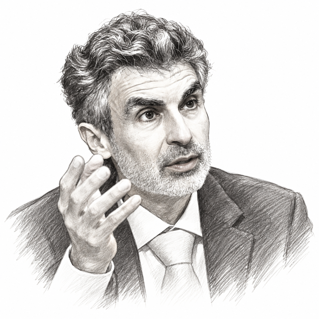
Instructor-supplied graphite-style portrait of Yoshua Bengio gesturing with one hand.

A pioneer of learned representations for language

2003 · Learn representations with the task

Word vectors and next-word probabilities are learned together with Ducharme, Vincent, and Jauvin. Paper

2014/2015 · Learn which source information to read

With Bahdanau and Cho, soft alignment becomes part of neural translation. Paper

2018 · ACM A.M. Turing Award

Shared with Geoffrey Hinton and Yann LeCun for breakthroughs in deep neural networks. ACM

Learn useful vectors, then learn how context should shape them.

References · recurrent learning and language representations

References · attention and Transformer encoders