Week 05 — Convolutions: Local Patterns and Shared Weights

Open in Colab. If GitHub access fails, download this notebook from the course Tutorials page and use File → Upload notebook in Colab.

Motivating question. How can a neural network recognize the same local pattern wherever it appears, without learning a separate weight for every location?

Teaching-source credit. The progression from a hand-calculated kernel response to a scanned response map is inspired by fastai’s Convolutional Neural Networks chapter. This tutorial uses original examples, notation, prose, code, and figures.

How to use this tutorial

This electronic chapter follows one investigation: how can a model detect a useful local pattern wherever it occurs, combine evidence across channels, and eventually classify an input? Run the cells in order, pause at each checkpoint, and read each figure after the labeled calculation that generates it.

The downloadable notebook is not a standalone bundle. It reads local images and MNIST-1D data from assets/, so run it from a checkout of the full course repository (from the repository root or tutorials/). The executed examples are deterministic and CPU-only; no runtime download or pickle loading is required.

Colab setup. Opening the notebook alone does not include its local assets. As an alternative to a full repository checkout, run the following in a new Colab code cell before the setup cells. It creates the expected course folders and fetches only the four public assets used here:

from pathlib import Path
from urllib.request import urlretrieve
import os

colab_root = Path("/content/Intro-to-ML-2026")
(colab_root / "tutorials").mkdir(parents=True, exist_ok=True)
asset_base = "https://avkornaev.github.io/Intro-to-ML-2026/assets/"
for asset in (
    "media/week05/chelsea-cat-rgb.png",
    "media/week05/mnist-train-00007-digit-3.png",
    "data/week05/mnist1d-official.npz",
    "data/week05/mnist1d-templates.npz",
):
    destination = colab_root / "assets" / asset
    destination.parent.mkdir(parents=True, exist_ok=True)
    urlretrieve(asset_base + asset, destination)
os.chdir(colab_root)

Learning objectives

By the end of the complete tutorial, students should be able to:

  • interpret grayscale and RGB images as batch-first tensors with explicit channel and spatial axes;
  • calculate one fixed-kernel response and explain how scanning produces a response map;
  • connect local connectivity and shared trainable weights to Week 04 gradient-based learning;
  • trace convolutional arithmetic across multiple input and output channels;
  • predict how padding, stride, pooling, and depth affect shapes and receptive fields;
  • trace a Conv1d stack’s receptive field and effective first-layer operator; and
  • design and interpret a fair MLP-versus-Conv1d comparison on MNIST-1D.

A compact notation guide

We introduce symbols where their operations first appear. Keep this short guide nearby:

Symbol Meaning
\(B\) batch size
\(C_{\mathrm{in}}, C_{\mathrm{out}}\) input and output channels
\(H,W\) (or \(T\) in 1D) spatial dimensions
\(k\), \(p\), \(s\) kernel size, padding, and stride, with axis subscripts when needed
\(\mathbf W^{(\ell)},\mathbf b^{(\ell)}\) layer parameters; \(\theta\) collects all trainable parameters
\(\mathbf z^{(\ell)}\) preactivations
\(\mathbf h^{(\ell)}=\phi(\mathbf z^{(\ell)})\) learned representations after activation, with \(\mathbf h^{(0)}=\mathbf X\)
\(\ell_i\), \(\mathcal L_{\mathcal B}\) one-example loss and mean mini-batch objective

We reserve \(K\) for the number of classes. PyTorch image batches use \((B,C_{\mathrm{in}},H,W)\); Conv1d inputs use \((B,C_{\mathrm{in}},T)\). PyTorch calls its unflipped cross-correlation operation “convolution.” A fixed kernel produces a response map; after trainable weights and an activation, we call the result a representation or activation map.

Tutorial map

Each scene answers the question raised by the previous one:

  1. Image tensors: where do pixels, channels, and batches live?
  2. Fixed kernels: how does one local calculation become a response map?
  3. Trainable shared kernels: what happens when the same weights are learned at every location?
  4. Multiple channels: how does each output channel combine all input channels?
  5. Spatial controls: how do padding, stride, pooling, and depth change the computation?
  6. A small CNN: how do those operations become a classifier?
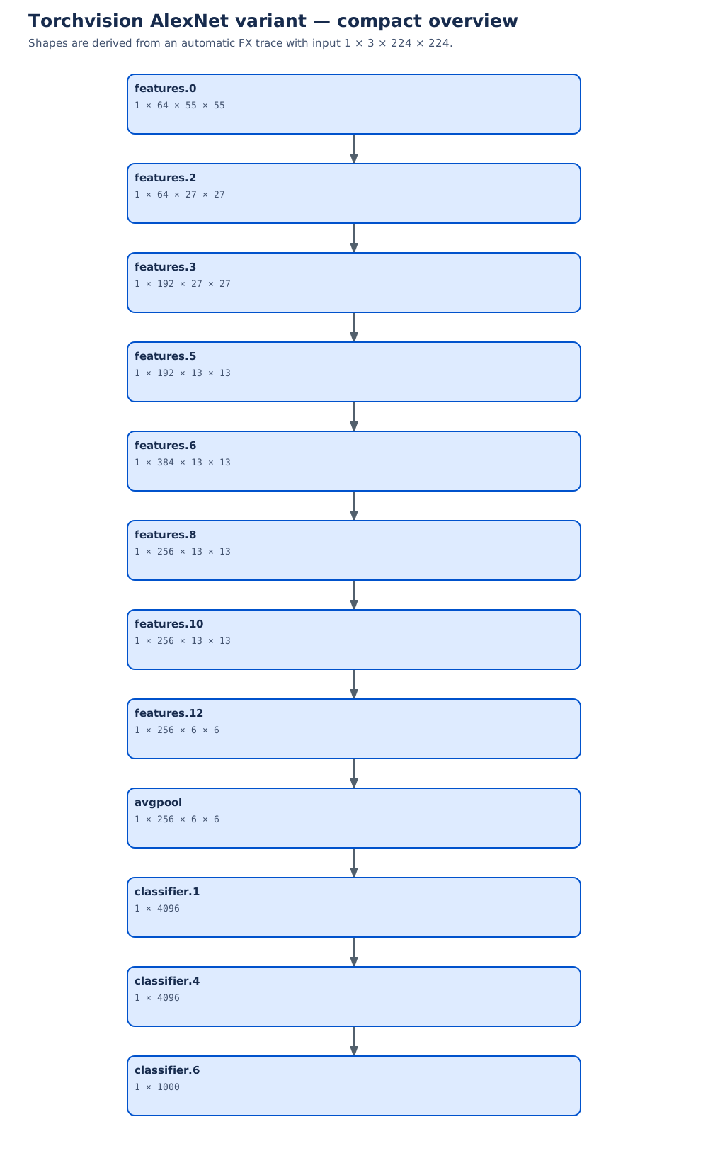
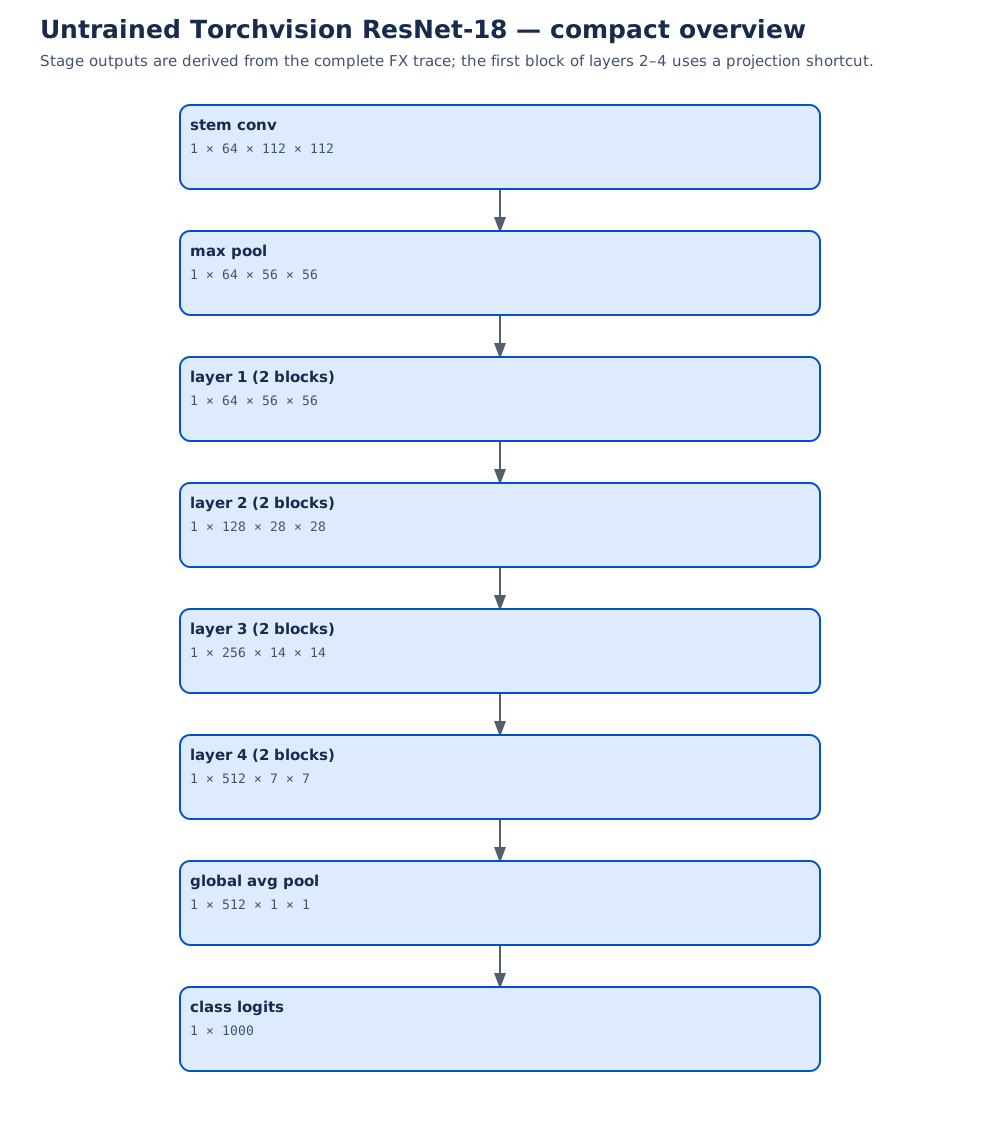
  7. Architecture reading: how do AlexNet and ResNet organize the same ideas at scale?
  8. MNIST-1D experiment: does local connectivity and weight sharing change learning under a controlled budget?

Setup

The notebook checks that it is inside the full repository before reading checked-in media and safe NumPy archives. If you downloaded only this .ipynb file, clone or download the repository first and open the notebook from that checkout.

from pathlib import Path
import hashlib
import time

import matplotlib.pyplot as plt
from matplotlib.animation import FuncAnimation, PillowWriter
from matplotlib.patches import Rectangle
from IPython.display import SVG, display
import numpy as np
import torch
import torch.nn as nn
import torch.nn.functional as F


def find_repo_root(start: Path) -> Path:
    for candidate in (start, *start.parents):
        if (candidate / "tutorials").is_dir() and (candidate / "assets").is_dir():
            return candidate
    raise RuntimeError("Run this notebook inside the Intro-to-ML-2026 repository.")


REPO_ROOT = find_repo_root(Path.cwd().resolve())
FIGURE_DIR = REPO_ROOT / "assets" / "figures" / "shared" / "week05"
MEDIA_DIR = REPO_ROOT / "assets" / "media" / "week05"
DATA_DIR = REPO_ROOT / "assets" / "data" / "week05"
FIGURE_DIR.mkdir(parents=True, exist_ok=True)
print(f"Figure exports: {FIGURE_DIR.relative_to(REPO_ROOT)}")
Figure exports: assets/figures/shared/week05

Auxiliary visualization and export code

The mathematical steps and PyTorch checks remain visible in the scenes below. Plot construction, styling, and animation export live in these collapsed cells so they do not interrupt the argument. In Colab, expand a cell if you want to modify a figure.

Show auxiliary style and export code
# @title Auxiliary: shared style, grid labels, and figure export
COURSE_NAVY = "#172033"
COURSE_BLUE = "#2457d6"
COURSE_GRAY = "#5f6878"
SIGNED_CMAP = "RdBu_r"
# Compatibility aliases for the unrevised Scene 3–5 plotting cells.
course_navy, course_blue, course_gray = COURSE_NAVY, COURSE_BLUE, COURSE_GRAY


def save_static_figure(fig, stem):
    svg_path = FIGURE_DIR / f"{stem}.svg"
    png_path = FIGURE_DIR / f"{stem}.png"
    fig.savefig(svg_path, bbox_inches="tight", facecolor="white")
    fig.savefig(png_path, dpi=180, bbox_inches="tight", facecolor="white")
    plt.close(fig)
    assert svg_path.stat().st_size > 0
    assert png_path.stat().st_size > 0
    print(f"saved {svg_path.relative_to(REPO_ROOT)}")
    print(f"saved {png_path.relative_to(REPO_ROOT)}")
    return svg_path, png_path


def write_grid_values(ax, values, *, decimals=2, threshold=None, fontsize=9,
                      background_values=None):
    for grid_row in range(values.shape[0]):
        for grid_column in range(values.shape[1]):
            value = float(values[grid_row, grid_column])
            value = 0.0 if abs(value) < 1e-12 else value
            text = f"{value:.{decimals}f}"
            if background_values is not None:
                background = float(background_values[grid_row, grid_column])
                color = "white" if background < 0.48 else COURSE_NAVY
            else:
                color = "white" if threshold is not None and abs(value) >= threshold else COURSE_NAVY
            ax.text(grid_column, grid_row, text, ha="center", va="center",
                    fontsize=fontsize, color=color)


def add_axis_labels(ax, height, width, *, row_label="row $h$", column_label="column $w$"):
    ax.set_xticks(range(width), labels=[str(c) for c in range(width)])
    ax.set_yticks(range(height), labels=[str(r) for r in range(height)])
    ax.set_xlabel(column_label, color=COURSE_GRAY)
    ax.set_ylabel(row_label, color=COURSE_GRAY)
Show auxiliary Scene 1 figure code
# @title Auxiliary: Scene 1 tensor figures
def export_tiny_tensor_layouts(gray_hw, rgb_hwc, rgb_chw, traced_row, traced_column):
    H, W = gray_hw.shape
    fig, axes = plt.subplots(2, 3, figsize=(11.5, 7.0), constrained_layout=True)
    gray_ax, rgb_ax, layout_ax = axes[0]
    channel_axes = axes[1]

    gray_ax.imshow(gray_hw.numpy(), cmap="gray", vmin=0, vmax=1)
    gray_ax.set_title(f"Grayscale values\n$(H,W)=({H},{W})$", color=COURSE_NAVY)
    write_grid_values(gray_ax, gray_hw, decimals=2, threshold=0.48)

    rgb_ax.imshow(rgb_hwc.numpy())
    rgb_ax.set_title(f"display layout\n$(H,W,C)=({H},{W},3)$", color=COURSE_NAVY)
    rgb_ax.add_patch(Rectangle((traced_column - 0.5, traced_row - 0.5), 1, 1,
                               fill=False, edgecolor=COURSE_BLUE, linewidth=3))

    layout_ax.axis("off")
    layout_ax.text(0.5, 0.72, "display", ha="center", color=COURSE_GRAY)
    layout_ax.text(0.5, 0.59, "$(H,W,C)$", ha="center", fontsize=18, color=COURSE_NAVY)
    layout_ax.annotate("move channel axis", xy=(0.5, 0.31), xytext=(0.5, 0.46),
                       ha="center", color=COURSE_BLUE,
                       arrowprops=dict(arrowstyle="->", color=COURSE_BLUE, lw=2))
    layout_ax.text(0.5, 0.17, "PyTorch image\n$(C,H,W)$", ha="center",
                   fontsize=15, color=COURSE_NAVY)

    for channel_index, (name, cmap) in enumerate(zip(("Red", "Green", "Blue"),
                                                      ("Reds", "Greens", "Blues"))):
        ax = channel_axes[channel_index]
        ax.imshow(rgb_chw[channel_index].numpy(), cmap=cmap, vmin=0, vmax=1)
        ax.set_title(f"{name} plane: CHW[{channel_index}, :, :]", color=COURSE_NAVY)
        ax.add_patch(Rectangle((traced_column - 0.5, traced_row - 0.5), 1, 1,
                               fill=False, edgecolor=COURSE_BLUE, linewidth=2))

    for ax in (gray_ax, rgb_ax, *channel_axes):
        add_axis_labels(ax, H, W)
    fig.suptitle("The same values can be indexed with different axis orders",
                 fontsize=16, fontweight="bold", color=COURSE_NAVY)
    return save_static_figure(fig, "01-image-tensor-layouts")


def export_rgb_channel_planes(photo_hwc):
    H, W, _ = photo_hwc.shape
    fig, axes = plt.subplots(1, 4, figsize=(12.0, 3.6), constrained_layout=True)
    axes[0].imshow(photo_hwc.numpy())
    axes[0].set_title(f"RGB image\n$(H,W,C)=({H},{W},3)$", color=COURSE_NAVY)
    for channel_index, (name, cmap) in enumerate(zip(("red", "green", "blue"),
                                                      ("Reds", "Greens", "Blues"))):
        axes[channel_index + 1].imshow(photo_hwc[:, :, channel_index].numpy(),
                                       cmap=cmap, vmin=0, vmax=1)
        axes[channel_index + 1].set_title(f"{name} plane\nHWC[:, :, {channel_index}]",
                                          color=COURSE_NAVY)
    for ax in axes:
        ax.set_xlabel("width $W$")
        ax.set_ylabel("height $H$")
        ax.set_xticks([])
        ax.set_yticks([])
    fig.suptitle("One RGB pixel has three channel values at one spatial location",
                 fontsize=16, fontweight="bold", color=COURSE_NAVY)
    return save_static_figure(fig, "01-rgb-channel-planes")
Show auxiliary Scene 2 figure and animation code
# @title Auxiliary: Scene 2 static key frame and animation

def export_three_kernel_bridge(image_hw, kernel_names, kernels_hw, responses_chw,
                               patch_origin):
    patch_row, patch_column = patch_origin
    fig = plt.figure(figsize=(11.5, 8.2), constrained_layout=True)
    grid = fig.add_gridspec(3, 3, width_ratios=(1.15, 1.0, 1.25))

    image_ax = fig.add_subplot(grid[:, 0])
    image_ax.imshow(image_hw.numpy(), cmap="gray", vmin=0, vmax=1)
    write_grid_values(image_ax, image_hw, decimals=0, background_values=image_hw, fontsize=9)
    image_ax.add_patch(Rectangle((patch_column - 0.5, patch_row - 0.5), 3, 3,
                                 fill=False, edgecolor=COURSE_BLUE, linewidth=3))
    image_ax.set_title("one $7\\times7$ image\nselected $3\\times3$ window", color=COURSE_NAVY)
    add_axis_labels(image_ax, 7, 7)

    for output_channel, name in enumerate(kernel_names):
        kernel_ax = fig.add_subplot(grid[output_channel, 1])
        kernel = kernels_hw[output_channel]
        kernel_limit = max(float(kernel.abs().max()), 1e-6)
        kernel_ax.imshow(kernel.numpy(), cmap=SIGNED_CMAP,
                         vmin=-kernel_limit, vmax=kernel_limit)
        write_grid_values(kernel_ax, kernel, decimals=2,
                          threshold=0.55 * kernel_limit, fontsize=9)
        kernel_ax.set_xticks(range(3)); kernel_ax.set_yticks(range(3))
        kernel_ax.set_title(f'{name} kernel\n$W[{output_channel},0,:,:]$',
                            color=COURSE_NAVY, fontsize=10)

        response_ax = fig.add_subplot(grid[output_channel, 2])
        response = responses_chw[output_channel]
        response_limit = max(float(response.abs().max()), 1e-6)
        artist = response_ax.imshow(response.numpy(), cmap=SIGNED_CMAP,
                                    vmin=-response_limit, vmax=response_limit)
        response_ax.add_patch(Rectangle((patch_column - 0.5, patch_row - 0.5), 1, 1,
                                        fill=False, edgecolor=COURSE_BLUE, linewidth=2.5))
        response_ax.set_title(
            f'output channel {output_channel}: {name}\n'
            f'R[{patch_row},{patch_column}]={response[patch_row, patch_column].item():+.3f}',
            color=COURSE_NAVY, fontsize=10,
        )
        response_ax.set_xlabel("output column"); response_ax.set_ylabel("output row")
        response_ax.set_xticks(range(5)); response_ax.set_yticks(range(5))
        fig.colorbar(artist, ax=response_ax, shrink=0.67, label="signed response")

    fig.suptitle("One image + three kernels = three response maps",
                 fontsize=16, fontweight="bold", color=COURSE_NAVY)
    return save_static_figure(fig, "02-three-kernel-bridge")


def export_digit_kernel_keyframe(image_hw, kernel_hw, response_hw, patch_row, patch_column,
                                 kernel_name):
    k_H, k_W = kernel_hw.shape
    patch = image_hw[patch_row:patch_row + k_H, patch_column:patch_column + k_W]
    products = patch * kernel_hw
    response_limit = max(float(response_hw.abs().max()), 1e-6)
    kernel_limit = max(float(kernel_hw.abs().max()), 1e-6)
    product_limit = max(float(products.abs().max()), 1e-6)

    fig, axes = plt.subplots(2, 3, figsize=(12.0, 7.5), constrained_layout=True)
    image_ax, patch_ax, kernel_ax, products_ax, sum_ax, response_ax = axes.flat
    image_ax.imshow(image_hw.numpy(), cmap="gray", vmin=0, vmax=1)
    image_ax.add_patch(Rectangle((patch_column - 0.5, patch_row - 0.5), k_W, k_H,
                                 fill=False, edgecolor=COURSE_BLUE, linewidth=2.5))
    image_ax.set_title("MNIST digit 3 and selected window", color=COURSE_NAVY)
    image_ax.set_xlabel("input column")
    image_ax.set_ylabel("input row")

    patch_ax.imshow(patch.numpy(), cmap="gray", vmin=0, vmax=1)
    write_grid_values(patch_ax, patch, decimals=2, fontsize=10,
                      background_values=patch)
    patch_ax.set_title(f"patch X[{patch_row}:{patch_row+3}, {patch_column}:{patch_column+3}]",
                       color=COURSE_NAVY)

    kernel_ax.imshow(kernel_hw.numpy(), cmap=SIGNED_CMAP,
                     vmin=-kernel_limit, vmax=kernel_limit)
    write_grid_values(kernel_ax, kernel_hw, decimals=2, threshold=0.55, fontsize=10)
    kernel_ax.set_title(f'kernel: "{kernel_name}"', color=COURSE_NAVY)

    products_ax.imshow(products.numpy(), cmap=SIGNED_CMAP,
                       vmin=-product_limit, vmax=product_limit)
    write_grid_values(products_ax, products, decimals=2, threshold=0.55, fontsize=10)
    products_ax.set_title("elementwise products", color=COURSE_NAVY)

    sum_ax.axis("off")
    sum_ax.text(0.5, 0.62, r"$R[r,c]=\sum_{u,v}X[r+u,c+v]W[u,v]$",
                ha="center", fontsize=14, color=COURSE_NAVY)
    sum_ax.text(0.5, 0.38, f"sum = {products.sum().item():+.3f}", ha="center",
                fontsize=19, fontweight="bold", color=COURSE_BLUE)

    response_artist = response_ax.imshow(response_hw.numpy(), cmap=SIGNED_CMAP,
                                          vmin=-response_limit, vmax=response_limit)
    response_ax.add_patch(Rectangle((patch_column - 0.5, patch_row - 0.5), 1, 1,
                                    fill=False, edgecolor=COURSE_BLUE, linewidth=2.5))
    response_ax.set_title(f"full response map {tuple(response_hw.shape)}", color=COURSE_NAVY)
    response_ax.set_xlabel("output column")
    response_ax.set_ylabel("output row")
    fig.colorbar(response_artist, ax=response_ax, shrink=0.75,
                 label="signed response (actual value)")
    for ax in (patch_ax, kernel_ax, products_ax):
        ax.set_xticks(range(3))
        ax.set_yticks(range(3))
    fig.suptitle("One local calculation fills one cell of the response map",
                 fontsize=16, fontweight="bold", color=COURSE_NAVY)
    paths = save_static_figure(fig, "02-mnist3-convolution-key-frame")
    display(SVG(filename=str(paths[0])))
    return paths


def export_digit_scan_animation(image_hw, kernel_hw, response_hw, scan_row, kernel_name):
    k_H, k_W = kernel_hw.shape
    H_out, W_out = response_hw.shape
    positions = [(scan_row, column) for column in range(W_out)]
    progress = torch.full_like(response_hw, float("nan"))
    cmap = plt.get_cmap(SIGNED_CMAP).copy()
    cmap.set_bad("#e7e9ee")
    response_limit = max(float(response_hw.abs().max()), 1e-6)

    fig, axes = plt.subplots(1, 4, figsize=(11.0, 3.4), constrained_layout=True)
    input_ax, patch_ax, products_ax, output_ax = axes
    input_ax.imshow(image_hw.numpy(), cmap="gray", vmin=0, vmax=1)
    window = Rectangle((-0.5, scan_row - 0.5), k_W, k_H, fill=False,
                       edgecolor=COURSE_BLUE, linewidth=2.5)
    input_ax.add_patch(window)
    input_ax.set_title(f'MNIST 3; kernel "{kernel_name}"')
    input_ax.set_xlabel("input column")
    input_ax.set_ylabel("input row")

    patch_artist = patch_ax.imshow(torch.zeros_like(kernel_hw).numpy(), cmap="gray", vmin=0, vmax=1)
    patch_ax.set_title("current patch")
    products_artist = products_ax.imshow(torch.zeros_like(kernel_hw).numpy(), cmap=SIGNED_CMAP,
                                          vmin=-1, vmax=1)
    products_ax.set_title("patch × kernel")
    output_artist = output_ax.imshow(progress.numpy(), cmap=cmap,
                                     vmin=-response_limit, vmax=response_limit)
    output_cell = Rectangle((-0.5, scan_row - 0.5), 1, 1, fill=False,
                            edgecolor=COURSE_BLUE, linewidth=2.5)
    output_ax.add_patch(output_cell)
    output_ax.set_xlabel("output column")
    output_ax.set_ylabel("output row")
    fig.colorbar(output_artist, ax=output_ax, shrink=0.72, label="signed response")

    def update(frame_index):
        row, column = positions[frame_index]
        patch = image_hw[row:row + k_H, column:column + k_W]
        products = patch * kernel_hw
        progress[row, column] = response_hw[row, column]
        window.set_xy((column - 0.5, row - 0.5))
        output_cell.set_xy((column - 0.5, row - 0.5))
        patch_artist.set_data(patch.numpy())
        products_artist.set_data(products.numpy())
        product_limit = max(float(products.abs().max()), 1e-6)
        products_artist.set_clim(-product_limit, product_limit)
        products_ax.set_title(f"products; sum={products.sum().item():+.2f}")
        output_artist.set_data(progress.numpy())
        output_ax.set_title(f"fill response[{row}, {column}]")
        return window, output_cell, patch_artist, products_artist, output_artist

    animation = FuncAnimation(fig, update, frames=len(positions), interval=220, blit=False)
    animation_path = FIGURE_DIR / "02-mnist3-convolution-scan.gif"
    animation.save(animation_path, writer=PillowWriter(fps=5), dpi=82)
    plt.close(fig)
    assert animation_path.stat().st_size > 0
    print(f"saved {animation_path.relative_to(REPO_ROOT)}")
    print(f"animation frames: {len(positions)}")
    return animation_path
Show auxiliary Scene 3 figure code
# @title Auxiliary: Scene 3 shared-weight figures
def export_shared_kernel_windows(input_1d, kernel_1d, response_1d):
    windows = input_1d.unfold(0, kernel_1d.numel(), 1)
    fig, axes = plt.subplots(1, 3, figsize=(10.5, 3.2), constrained_layout=True)
    colours = ("#dbe7ff", "#ffe7c2")
    for location, ax in enumerate(axes):
        ax.axis("off")
        ax.set_xlim(-0.15, 2.15)
        ax.set_ylim(-0.25, 1.55)
        for offset in range(2):
            ax.add_patch(Rectangle((offset, 0.45), 0.9, 0.72,
                                   facecolor=colours[offset], edgecolor=COURSE_NAVY))
            ax.text(offset + 0.45, 0.81,
                    f"$w_{offset}x_{{{location + offset}}}$\n"
                    f"$={kernel_1d[offset].item():g}\\cdot{windows[location, offset].item():g}$",
                    ha="center", va="center", fontsize=12, color=COURSE_NAVY)
        ax.text(0.9, 0.16, f"$z_{location}={response_1d[location].item():g}$",
                ha="center", fontsize=14, fontweight="bold", color=COURSE_BLUE)
        ax.set_title(f"window {location}: $[x_{location},x_{location + 1}]$",
                     color=COURSE_NAVY, fontsize=12)
    fig.suptitle("The same two kernel parameters are reused at all three locations",
                 fontsize=15, fontweight="bold", color=COURSE_NAVY)
    return save_static_figure(fig, "03-shared-kernel-windows")


def export_shared_weights_sparse_operator(input_1d, kernel_1d, response_1d):
    fig, ax = plt.subplots(figsize=(9.5, 4.8), constrained_layout=True)
    ax.set_xlim(-0.9, 5.8)
    ax.set_ylim(3.5, -0.7)
    ax.axis("off")
    shared_colours = {"w_0": "#dbe7ff", "w_1": "#ffe7c2", "0": "#f3f4f6"}
    labels = [
        [("w_0", "2"), ("w_1", "-1"), ("0", "0"), ("0", "0")],
        [("0", "0"), ("w_0", "2"), ("w_1", "-1"), ("0", "0")],
        [("0", "0"), ("0", "0"), ("w_0", "2"), ("w_1", "-1")],
    ]
    for matrix_row, row_labels in enumerate(labels):
        for matrix_column, (name, value) in enumerate(row_labels):
            ax.add_patch(Rectangle((matrix_column, matrix_row), 1, 1,
                                   facecolor=shared_colours[name], edgecolor=COURSE_NAVY,
                                   linewidth=1.2))
            text = value if name == "0" else f"${name}={value}$"
            ax.text(matrix_column + 0.5, matrix_row + 0.5, text,
                    ha="center", va="center", fontsize=12)
    ax.text(-0.28, 1.5, "effective\noperator", ha="center", va="center", color=COURSE_GRAY)
    ax.text(4.3, 1.5, r"$\times\ [1,2,3,4]^\mathsf{T}$", ha="left", va="center", fontsize=14)
    ax.text(5.45, 1.5, r"$=[0,1,2]^\mathsf{T}$", ha="left", va="center", fontsize=14)
    ax.text(2.0, 3.25, r"same $w_0$ appears 3 times; same $w_1$ appears 3 times",
            ha="center", color=COURSE_BLUE, fontsize=12)
    ax.set_title("A local scan is a sparse linear operation with tied weights",
                 fontsize=15, fontweight="bold", color=COURSE_NAVY)
    return save_static_figure(fig, "03-shared-weights-sparse-operator")
Show auxiliary Scene 4–5 figure code
# @title Auxiliary: Scene 4–5 explanatory figures
def draw_numeric_grid(ax, values, title, *, decimals=2):
    limit = max(float(values.abs().max()), 1e-6)
    ax.imshow(values.numpy(), cmap=SIGNED_CMAP, vmin=-limit, vmax=limit)
    write_grid_values(ax, values, decimals=decimals, threshold=0.55 * limit, fontsize=8)
    ax.set_xticks(range(values.shape[1]))
    ax.set_yticks(range(values.shape[0]))
    ax.set_title(title, fontsize=10, color=COURSE_NAVY)


def export_color_convolution_keyframe(photo_hwc, patch_origin, weights, biases,
                                      contributions, outputs, responses, filter_names):
    patch_row, patch_column = patch_origin
    fig = plt.figure(figsize=(14.0, 8.5), constrained_layout=True)
    grid = fig.add_gridspec(3, 5, height_ratios=(1.35, 1, 1))
    image_ax = fig.add_subplot(grid[0, :2])
    image_ax.imshow(photo_hwc.numpy())
    image_ax.add_patch(Rectangle((patch_column - 0.5, patch_row - 0.5), 3, 3,
                                 fill=False, edgecolor=COURSE_BLUE, linewidth=2.4))
    image_ax.set_title("Chelsea RGB input; exact $3\\times3$ patch outlined", color=COURSE_NAVY)
    image_ax.set_xticks([]); image_ax.set_yticks([])

    response_limit = max(float(responses.abs().max()), 1e-6)
    for output_channel in range(2):
        ax = fig.add_subplot(grid[0, output_channel + 2])
        artist = ax.imshow(responses[output_channel].numpy(), cmap=SIGNED_CMAP,
                           vmin=-response_limit, vmax=response_limit)
        ax.add_patch(Rectangle((patch_column - 0.5, patch_row - 0.5), 1, 1,
                               fill=False, edgecolor=COURSE_BLUE, linewidth=2))
        ax.set_title(f"output {output_channel}: {filter_names[output_channel]}\n"
                     f"signed response {tuple(responses[output_channel].shape)}",
                     fontsize=10, color=COURSE_NAVY)
        ax.set_xticks([]); ax.set_yticks([])
    color_ax = fig.add_subplot(grid[0, 4])
    color_ax.axis("off")
    fig.colorbar(artist, ax=color_ax, fraction=0.8, label="signed response (not normalized)")

    channel_names = ("red", "green", "blue")
    for output_channel in range(2):
        label_ax = fig.add_subplot(grid[output_channel + 1, 0])
        label_ax.axis("off")
        label_ax.text(0.02, 0.72, f"output channel {output_channel}", fontsize=13,
                      fontweight="bold", color=COURSE_NAVY)
        label_ax.text(0.02, 0.48, filter_names[output_channel], fontsize=11,
                      color=COURSE_BLUE, wrap=True)
        label_ax.text(0.02, 0.17, "three input-channel slices $\\rightarrow$ one output",
                      fontsize=9, color=COURSE_GRAY)
        for input_channel, channel_name in enumerate(channel_names):
            ax = fig.add_subplot(grid[output_channel + 1, input_channel + 1])
            draw_numeric_grid(
                ax, weights[output_channel, input_channel],
                f"{channel_name} slice $W[{output_channel},{input_channel}]$\n"
                f"patch contribution {contributions[output_channel, input_channel].item():+.4f}",
                decimals=2,
            )
        total_ax = fig.add_subplot(grid[output_channel + 1, 4])
        total_ax.axis("off")
        terms = " + ".join(f"{value.item():+.4f}" for value in contributions[output_channel])
        total_ax.text(0.5, 0.68, "channel sums + bias", ha="center", color=COURSE_GRAY)
        total_ax.text(0.5, 0.47, terms, ha="center", fontsize=9, color=COURSE_NAVY)
        total_ax.text(0.5, 0.30, f"+ {biases[output_channel].item():+.3f}",
                      ha="center", fontsize=10, color=COURSE_NAVY)
        total_ax.text(0.5, 0.10, f"= {outputs[output_channel].item():+.4f}",
                      ha="center", fontsize=14, fontweight="bold", color=COURSE_BLUE)
    fig.suptitle("Each output filter has its own RGB slices; every slice contributes",
                 fontsize=16, fontweight="bold", color=COURSE_NAVY)
    return save_static_figure(fig, "04-color-convolution-key-frame")


def export_spatial_controls_keyframes(image, kernel, cases):
    fig, axes = plt.subplots(3, 3, figsize=(12.5, 10.0), constrained_layout=True)
    colours = (COURSE_BLUE, "#d97706", "#7c3aed")
    for row, case in enumerate(cases):
        name, response, padding, stride, starts = case
        padded = F.pad(image.reshape(1, 1, *image.shape),
                       (padding, padding, padding, padding))[0, 0]
        input_ax, parameter_ax, output_ax = axes[row]
        input_ax.imshow(padded.numpy(), cmap="gray", vmin=0, vmax=1)
        if padding:
            input_ax.add_patch(Rectangle((padding - 0.5, padding - 0.5), 28, 28,
                                         fill=False, edgecolor="#9ca3af", linestyle="--"))
        for colour, (start_row, start_column) in zip(colours, starts):
            input_ax.add_patch(Rectangle((start_column - 0.5, start_row - 0.5), 3, 3,
                                         fill=False, edgecolor=colour, linewidth=2))
        input_ax.set_title(f"{name}: {'padded ' if padding else ''}input {tuple(padded.shape)}")
        input_ax.set_xticks([]); input_ax.set_yticks([])

        parameter_ax.axis("off")
        parameter_ax.text(0.5, 0.78, "$k=3$", ha="center", fontsize=15, color=COURSE_NAVY)
        parameter_ax.text(0.5, 0.58, f"$p={padding}$", ha="center", fontsize=15, color=COURSE_NAVY)
        parameter_ax.text(0.5, 0.38, f"$s={stride}$", ha="center", fontsize=15, color=COURSE_NAVY)
        parameter_ax.annotate("window starts\nmap to output cells", xy=(0.92, 0.5),
                              xytext=(0.08, 0.5), ha="center", va="center",
                              arrowprops=dict(arrowstyle="->", color=COURSE_BLUE, lw=2),
                              color=COURSE_GRAY)

        height, width = response.shape
        output_ax.set_xlim(-1, 29); output_ax.set_ylim(29, -1); output_ax.set_aspect("equal")
        output_ax.add_patch(Rectangle((-0.5, -0.5), width, height,
                                      facecolor="#f3f4f6", edgecolor=COURSE_NAVY, linewidth=2))
        output_positions = [(start_row // stride, start_column // stride)
                            for start_row, start_column in starts]
        for colour, (out_row, out_column) in zip(colours, output_positions):
            output_ax.add_patch(Rectangle((out_column - 0.5, out_row - 0.5), 1, 1,
                                          facecolor=colour, edgecolor=colour))
        output_ax.set_title(f"output grid {height}×{width}\n{height * width} evaluated windows")
        output_ax.set_xticks([]); output_ax.set_yticks([])
    fig.suptitle("Padding changes the input domain; stride changes which starts are evaluated",
                 fontsize=15, fontweight="bold", color=COURSE_NAVY)
    return save_static_figure(fig, "05-spatial-controls-key-frames")


def export_pooling_window(window, winner, winner_offset, output_index):
    fig, axes = plt.subplots(1, 3, figsize=(8.7, 2.8), constrained_layout=True,
                             gridspec_kw={"width_ratios": (1.2, 0.7, 1.2)})
    draw_numeric_grid(axes[0], window, "four signed responses", decimals=3)
    axes[0].add_patch(Rectangle((winner_offset[1] - 0.5, winner_offset[0] - 0.5), 1, 1,
                                fill=False, edgecolor="#d97706", linewidth=3))
    axes[1].axis("off")
    axes[1].annotate("choose max", xy=(0.95, 0.5), xytext=(0.05, 0.5),
                     arrowprops=dict(arrowstyle="->", lw=2, color=COURSE_BLUE),
                     va="center", color=COURSE_GRAY)
    axes[2].axis("off")
    axes[2].add_patch(Rectangle((0.2, 0.25), 0.6, 0.5, facecolor="#dbe7ff",
                                edgecolor=COURSE_BLUE, linewidth=2))
    axes[2].text(0.5, 0.52, f"{winner.item():+.3f}", ha="center", va="center",
                 fontsize=17, fontweight="bold", color=COURSE_NAVY)
    axes[2].text(0.5, 0.12, f"pooled output {output_index}", ha="center", color=COURSE_GRAY)
    fig.suptitle("Max pooling keeps one value and discards the other three",
                 fontsize=14, fontweight="bold", color=COURSE_NAVY)
    return save_static_figure(fig, "05-max-pooling-window")


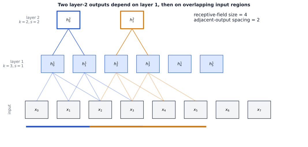
def export_receptive_field_trace(traced, size, spacing):
    fig, ax = plt.subplots(figsize=(11.0, 5.2), constrained_layout=True)
    ax.axis("off"); ax.set_xlim(-0.7, 8.8); ax.set_ylim(-0.6, 3.1)
    layer_y = {"input": 0.1, "layer1": 1.35, "layer2": 2.55}
    for index in range(8):
        ax.add_patch(Rectangle((index, layer_y["input"]), 0.72, 0.48,
                               facecolor="#f3f4f6", edgecolor=COURSE_NAVY))
        ax.text(index + 0.36, layer_y["input"] + 0.24, f"$x_{index}$", ha="center", va="center")
    for index in range(6):
        ax.add_patch(Rectangle((index + 0.5, layer_y["layer1"]), 0.72, 0.48,
                               facecolor="#dbe7ff", edgecolor=COURSE_BLUE))
        ax.text(index + 0.86, layer_y["layer1"] + 0.24, f"$h^1_{index}$", ha="center", va="center")
    for index, colour in zip((0, 1), (COURSE_BLUE, "#d97706")):
        x = 1.0 + 2 * index
        ax.add_patch(Rectangle((x, layer_y["layer2"]), 0.72, 0.48,
                               facecolor="white", edgecolor=colour, linewidth=2.5))
        ax.text(x + 0.36, layer_y["layer2"] + 0.24, f"$h^2_{index}$", ha="center", va="center")
        for middle in (2 * index, 2 * index + 1):
            middle_x = middle + 0.86
            ax.plot([x + 0.36, middle_x], [layer_y["layer2"], layer_y["layer1"] + 0.48],
                    color=colour, alpha=0.8)
            for source in range(middle, middle + 3):
                ax.plot([middle_x, source + 0.36], [layer_y["layer1"], layer_y["input"] + 0.48],
                        color=colour, alpha=0.35)
        coords = traced[index]
        ax.plot([coords[0] + 0.05, coords[-1] + 0.67], [-0.12, -0.12],
                color=colour, linewidth=4)
    ax.text(-0.55, 0.35, "input", rotation=90, va="center", color=COURSE_GRAY)
    ax.text(-0.05, 1.59, "layer 1\n$k=3,s=1$", ha="right", va="center", color=COURSE_GRAY)
    ax.text(0.45, 2.79, "layer 2\n$k=2,s=2$", ha="right", va="center", color=COURSE_GRAY)
    ax.text(5.3, 2.75, f"receptive-field size = {size}\nadjacent-output spacing = {spacing}",
            color=COURSE_NAVY, fontsize=12)
    ax.set_title("Two layer-2 outputs depend on layer 1, then on overlapping input regions",
                 fontweight="bold", color=COURSE_NAVY)
    return save_static_figure(fig, "05-receptive-field-trace")
Show auxiliary Scene 6 figure code
# @title Auxiliary: Scene 6 structural CNN figure
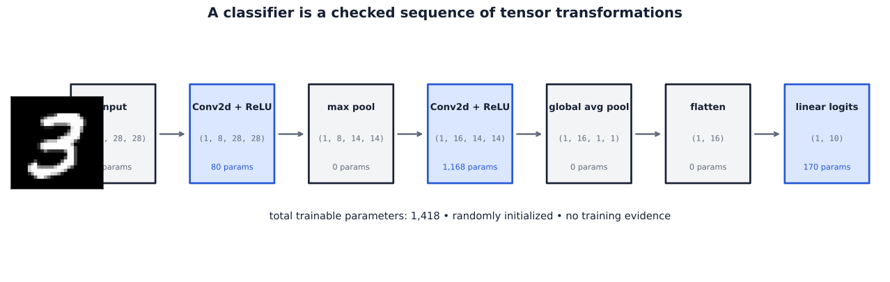
def export_cnn_architecture(image_hw, ledger):
    stages = [
        ("input", ledger[0][1], 0),
        ("Conv2d + ReLU", ledger[1][1], ledger[1][2]),
        ("max pool", ledger[3][1], 0),
        ("Conv2d + ReLU", ledger[4][1], ledger[4][2]),
        ("global avg pool", ledger[6][1], 0),
        ("flatten", ledger[7][1], 0),
        ("linear logits", ledger[8][1], ledger[8][2]),
    ]
    fig, ax = plt.subplots(figsize=(13.2, 4.1), constrained_layout=True)
    ax.axis("off"); ax.set_xlim(-0.8, 13.2); ax.set_ylim(-0.6, 3.1)
    image_ax = ax.inset_axes([0.005, 0.31, 0.105, 0.43])
    image_ax.imshow(image_hw.numpy(), cmap="gray", vmin=0, vmax=1)
    image_ax.set_xticks([]); image_ax.set_yticks([])
    x_positions = [0.9, 2.8, 4.7, 6.6, 8.5, 10.4, 12.3]
    for index, ((name, shape, parameters), x) in enumerate(zip(stages, x_positions)):
        width = 1.35
        face = "#f3f4f6" if parameters == 0 else "#dbe7ff"
        ax.add_patch(Rectangle((x - width / 2, 0.75), width, 1.45,
                               facecolor=face, edgecolor=COURSE_BLUE if parameters else COURSE_NAVY,
                               linewidth=2))
        ax.text(x, 1.86, name, ha="center", va="center", fontsize=10,
                fontweight="bold", color=COURSE_NAVY, wrap=True)
        ax.text(x, 1.40, str(shape), ha="center", va="center", fontsize=8.5,
                family="monospace", color=COURSE_GRAY)
        ax.text(x, 0.98, f"{parameters:,} params" if parameters else "0 params",
                ha="center", va="center", fontsize=8.5, color=COURSE_BLUE if parameters else COURSE_GRAY)
        if index < len(stages) - 1:
            ax.annotate("", xy=(x_positions[index + 1] - 0.72, 1.47),
                        xytext=(x + 0.72, 1.47),
                        arrowprops=dict(arrowstyle="->", lw=1.8, color=COURSE_GRAY))
    ax.text(6.6, 0.22, "total trainable parameters: 1,418 • randomly initialized • no training evidence",
            ha="center", fontsize=11, color=COURSE_NAVY)
    ax.set_title("A classifier is a checked sequence of tensor transformations",
                 fontsize=15, fontweight="bold", color=COURSE_NAVY)
    return save_static_figure(fig, "06-cnn-architecture")
Show auxiliary MNIST-1D plotting and export code
# @title Auxiliary: MNIST-1D figures and routine experiment bookkeeping
def export_mnist1d_templates_and_variation(template_x, template_t, template_y,
                                           signals, labels):
    fig = plt.figure(figsize=(13.0, 8.5), constrained_layout=True)
    outer = fig.add_gridspec(3, 5, height_ratios=(1, 1, 1.15))
    for digit in range(10):
        ax = fig.add_subplot(outer[digit // 5, digit % 5])
        ax.plot(template_t, template_x[digit], color=COURSE_NAVY, linewidth=2)
        ax.axhline(0, color="#c7cbd3", linewidth=0.8)
        ax.set_title(f"template {digit}", color=COURSE_NAVY)
        ax.set_xticks([]); ax.set_yticks([])
    class_three_indices = torch.nonzero(labels == 3).flatten()[:3]
    focus_axes = [fig.add_subplot(outer[2, column]) for column in range(4)]
    focus_axes[0].plot(template_t, template_x[3], color=COURSE_NAVY, linewidth=2.4)
    focus_axes[0].set_title("clean template 3\n12 source points", color=COURSE_NAVY)
    focus_axes[0].set_xlabel("template coordinate")
    for ax, index in zip(focus_axes[1:], class_three_indices):
        ax.plot(range(signals.shape[1]), signals[index].numpy(), color=COURSE_BLUE, linewidth=1.6)
        ax.set_title(f"supplied class 3\ntrain index {int(index)}", color=COURSE_NAVY)
        ax.set_xlabel("signal position $t$")
    for ax in focus_axes:
        ax.axhline(0, color="#c7cbd3", linewidth=0.8)
        ax.set_ylabel("value")
    note_ax = fig.add_subplot(outer[2, 4])
    note_ax.axis("off")
    note_ax.text(0.03, 0.78, "Examples may differ through", fontweight="bold", color=COURSE_NAVY)
    note_ax.text(0.03, 0.62, "• padding / translation\n• scaling and shear\n• correlated + iid noise",
                 va="top", color=COURSE_GRAY, linespacing=1.5)
    note_ax.text(0.03, 0.17, "These are generation mechanisms,\nnot recovered parameters for\nany displayed sample.",
                 color="#9b2c2c", va="top")
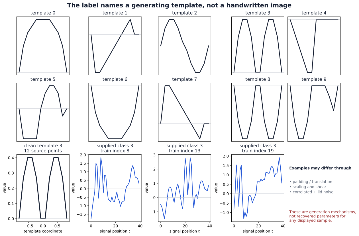
    fig.suptitle("The label names a generating template, not a handwritten image",
                 fontsize=16, fontweight="bold", color=COURSE_NAVY)
    return save_static_figure(fig, "08-mnist1d-templates-and-variation")


def export_effective_operators(conv_operator, dense_weights, kernel_values):
    fig, axes = plt.subplots(1, 2, figsize=(11.0, 4.4), constrained_layout=True)
    limit = max(float(conv_operator.abs().max()), float(dense_weights.abs().max()), 1e-6)
    axes[0].imshow(conv_operator.numpy(), cmap=SIGNED_CMAP, vmin=-limit, vmax=limit, aspect="auto")
    axes[0].set_title("initialized Conv1d channel: $40\\times40$ effective operator")
    axes[0].set_xlabel("input position"); axes[0].set_ylabel("output position")
    axes[0].text(0.02, 0.98, "initialized kernel = [" + ", ".join(f"{v:+.2f}" for v in kernel_values) + "]",
                 transform=axes[0].transAxes, va="top", fontsize=8.5,
                 bbox=dict(facecolor="white", alpha=0.88, edgecolor="none"))
    dense_artist = axes[1].imshow(dense_weights.numpy(), cmap=SIGNED_CMAP,
                                  vmin=-limit, vmax=limit, aspect="auto")
    axes[1].set_title("initialized MLP first layer: independent dense weights")
    axes[1].set_xlabel("input position"); axes[1].set_ylabel("hidden unit")
    fig.colorbar(dense_artist, ax=axes, shrink=0.75, label="initialized stored/effective weight")
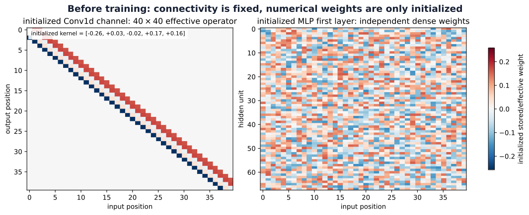
    fig.suptitle("Before training: connectivity is fixed, numerical weights are only initialized",
                 fontsize=14, fontweight="bold", color=COURSE_NAVY)
    return save_static_figure(fig, "08-mnist1d-effective-operators")


def export_learning_curves(histories):
    fig, axes = plt.subplots(2, 2, figsize=(10.5, 7.0), constrained_layout=True)
    for name, history in histories.items():
        epochs = range(1, len(history["train_loss"]) + 1)
        axes[0, 0].plot(epochs, history["train_loss"], label=name)
        axes[0, 1].plot(epochs, history["validation_loss"], label=name)
        axes[1, 0].plot(epochs, history["train_accuracy"], label=name)
        axes[1, 1].plot(epochs, history["validation_accuracy"], label=name)
    titles = (("training loss", "validation loss"),
              ("training accuracy", "validation accuracy"))
    for row in range(2):
        for column in range(2):
            axes[row, column].set_title(titles[row][column])
            axes[row, column].set_xlabel("epoch")
            axes[row, column].grid(alpha=0.2)
            axes[row, column].legend()
    axes[1, 0].set_ylim(0, 1); axes[1, 1].set_ylim(0, 1)
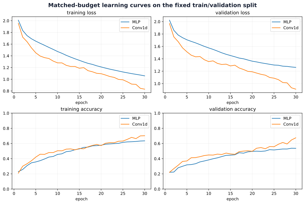
    fig.suptitle("Matched-budget learning curves on the fixed train/validation split",
                 fontsize=14, fontweight="bold", color=COURSE_NAVY)
    return save_static_figure(fig, "08-mnist1d-learning-curves")


def choose_comparison_examples(labels, mlp_predictions, conv_predictions):
    masks = {
        "both correct": (mlp_predictions == labels) & (conv_predictions == labels),
        "only MLP wrong": (mlp_predictions != labels) & (conv_predictions == labels),
        "only Conv1d wrong": (mlp_predictions == labels) & (conv_predictions != labels),
        "both wrong": (mlp_predictions != labels) & (conv_predictions != labels),
    }
    selected, used = [], set()
    for category, mask in masks.items():
        candidates = torch.nonzero(mask).flatten().tolist()
        if candidates:
            index = candidates[0]
            selected.append((category, index, False))
            used.add(index)
        else:
            alternatives = [i for i in range(len(labels)) if i not in used]
            index = alternatives[0]
            selected.append((f"{category} unavailable; fallback", index, True))
            used.add(index)
    return selected, {name: int(mask.sum()) for name, mask in masks.items()}


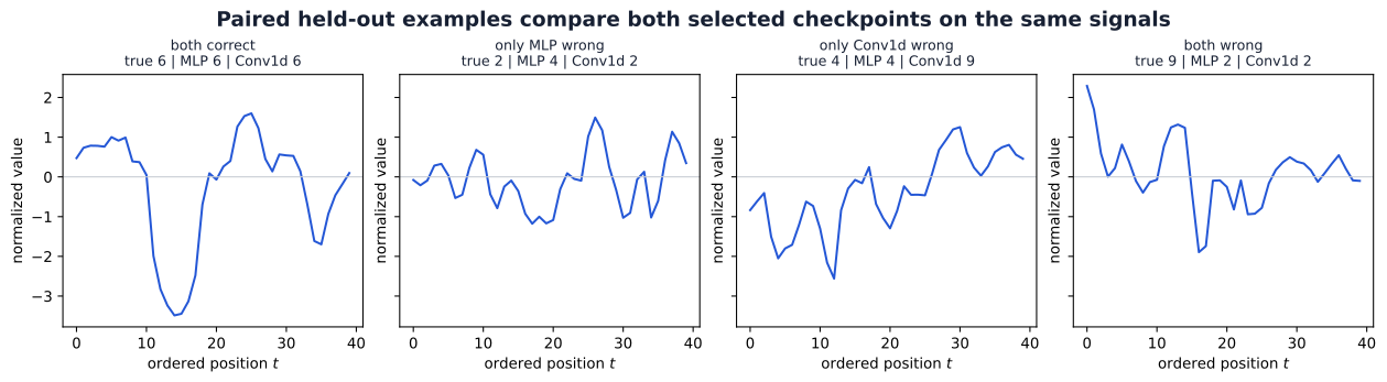
def export_comparison_examples(signals, labels, mlp_predictions, conv_predictions, selected):
    fig, axes = plt.subplots(1, 4, figsize=(13.0, 3.5), sharex=True, sharey=True,
                             constrained_layout=True)
    for ax, (category, index, is_fallback) in zip(axes, selected):
        ax.plot(range(signals.shape[1]), signals[index].numpy(), color=COURSE_BLUE)
        ax.axhline(0, color="#c7cbd3", linewidth=0.8)
        prefix = "fallback\n" if is_fallback else ""
        ax.set_title(prefix + category + f"\ntrue {int(labels[index])} | "
                     f"MLP {int(mlp_predictions[index])} | Conv1d {int(conv_predictions[index])}",
                     fontsize=9.5, color=COURSE_NAVY)
        ax.set_xlabel("ordered position $t$")
        ax.set_ylabel("normalized value")
    fig.suptitle("Paired held-out examples compare both selected checkpoints on the same signals",
                 fontsize=14, fontweight="bold", color=COURSE_NAVY)
    return save_static_figure(fig, "08-mnist1d-errors")

Scene 1 — Image tensors: pixels, channels, and shapes

Question. Which tensor axis names a pixel’s spatial location, and which axis names the value stored at that location?

Start with tiny exact arrays. A grayscale image has one intensity per location; an RGB image has red, green, and blue values at the same \((h,w)\) location.

Tiny tensors with labeled axes

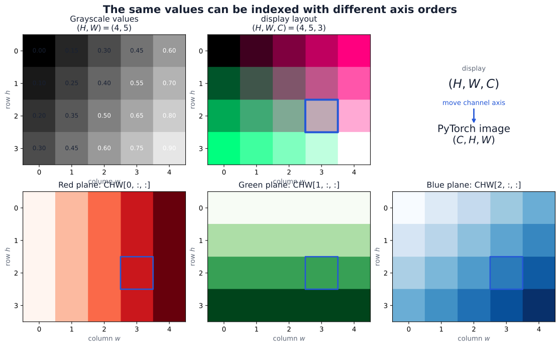
Display tools commonly use \((H,W,C)\) for RGB data. PyTorch image layers use \((C,H,W)\) for one image and \((B,C,H,W)\) for a batch. The operation below moves an axis; it does not change any pixel value.

H, W, C = 4, 5, 3
gray_hw = torch.tensor(
    [[0.00, 0.15, 0.30, 0.45, 0.60],
     [0.10, 0.25, 0.40, 0.55, 0.70],
     [0.20, 0.35, 0.50, 0.65, 0.80],
     [0.30, 0.45, 0.60, 0.75, 0.90]],
    dtype=torch.float32,
)
row_values = torch.linspace(0.0, 1.0, H).unsqueeze(1).expand(H, W)
column_values = torch.linspace(0.0, 1.0, W).unsqueeze(0).expand(H, W)
rgb_hwc = torch.stack((column_values, row_values,
                       0.5 * (row_values + column_values)), dim=-1)

assert gray_hw.shape == (H, W)
assert rgb_hwc.shape == (H, W, C)
assert torch.all((0 <= rgb_hwc) & (rgb_hwc <= 1))
print(f"grayscale: {tuple(gray_hw.shape)} = (H, W)")
print(f"RGB display tensor: {tuple(rgb_hwc.shape)} = (H, W, C)")
print("pixel HWC[2, 3, :] =", rgb_hwc[2, 3].tolist())
grayscale: (4, 5) = (H, W)
RGB display tensor: (4, 5, 3) = (H, W, C)
pixel HWC[2, 3, :] = [0.75, 0.6666666269302368, 0.7083333134651184]

Prediction checkpoint — follow one value

The red value at zero-based location \((h,w)=(2,3)\) is rgb_hwc[2, 3, 0].

Before running the next cell, predict its index after conversion to \((C,H,W)\), the resulting single-image shape, and the shape after stacking two images into a batch.

rgb_chw = rgb_hwc.permute(2, 0, 1).contiguous()
gray_chw = gray_hw.unsqueeze(0)
rgb_bchw = torch.stack((rgb_chw, torch.flip(rgb_chw, dims=(2,))), dim=0)
gray_bchw = gray_chw.unsqueeze(0)

row, column, channel = 2, 3, 0
assert rgb_chw.shape == (C, H, W)
assert rgb_bchw.shape == (2, C, H, W)
assert gray_chw.shape == (1, H, W)
assert gray_bchw.shape == (1, 1, H, W)
torch.testing.assert_close(rgb_hwc[row, column, channel],
                           rgb_chw[channel, row, column], rtol=0, atol=0)
torch.testing.assert_close(rgb_hwc[row, column, channel],
                           rgb_bchw[0, channel, row, column], rtol=0, atol=0)

print(f"single RGB image: {tuple(rgb_chw.shape)} = (C, H, W)")
print(f"batch of two:     {tuple(rgb_bchw.shape)} = (B, C, H, W)")
print(f"same red value: HWC[2,3,0] = CHW[0,2,3] = {rgb_chw[0,2,3].item():.2f}")
single RGB image: (3, 4, 5) = (C, H, W)
batch of two:     (2, 3, 4, 5) = (B, C, H, W)
same red value: HWC[2,3,0] = CHW[0,2,3] = 0.75

The spatial indices remain \((h,w)=(2,3)\) while the channel index moves from the last axis to the first. A batch adds a new leading axis; it does not merge images with channels.

export_tiny_tensor_layouts(gray_hw, rgb_hwc, rgb_chw, row, column)
saved assets/figures/shared/week05/01-image-tensor-layouts.svg
saved assets/figures/shared/week05/01-image-tensor-layouts.png
(PosixPath('/Users/alexeykornaev/Documents/GitHub/Intro-to-ML-2026/assets/figures/shared/week05/01-image-tensor-layouts.svg'),
 PosixPath('/Users/alexeykornaev/Documents/GitHub/Intro-to-ML-2026/assets/figures/shared/week05/01-image-tensor-layouts.png'))
A four-by-five grayscale value grid and a small RGB tensor appear beside red, green, and blue channel planes. The same pixel is outlined before and after the channel axis moves.
Figure 1: A four-by-five grayscale value grid and a small RGB tensor appear beside red, green, and blue channel planes. The same pixel is outlined before and after the channel axis moves.

A genuine RGB image

The same layout rules apply to a photograph. This local image is a resized copy of scikit-image’s “Chelsea” photograph, released CC0 by photographer Stefan van der Walt; the repository records the exact source and transformation in assets/media/week05/README.md.

rgb_photo_hwc = torch.from_numpy(
    plt.imread(MEDIA_DIR / "chelsea-cat-rgb.png").copy()
).to(torch.float32)
rgb_photo_chw = rgb_photo_hwc.permute(2, 0, 1).contiguous()
rgb_photo_bchw = rgb_photo_chw.unsqueeze(0)
photo_H, photo_W, photo_C = rgb_photo_hwc.shape

assert (photo_H, photo_W, photo_C) == (120, 180, 3)
assert rgb_photo_chw.shape == (3, 120, 180)
assert rgb_photo_bchw.shape == (1, 3, 120, 180)
torch.testing.assert_close(rgb_photo_hwc[60, 90, 1], rgb_photo_chw[1, 60, 90], rtol=0, atol=0)
print(f"display: {tuple(rgb_photo_hwc.shape)} = (H, W, C)")
print(f"PyTorch: {tuple(rgb_photo_chw.shape)} = (C, H, W)")
print(f"batched: {tuple(rgb_photo_bchw.shape)} = (B, C, H, W)")
display: (120, 180, 3) = (H, W, C)
PyTorch: (3, 120, 180) = (C, H, W)
batched: (1, 3, 120, 180) = (B, C, H, W)
export_rgb_channel_planes(rgb_photo_hwc)
saved assets/figures/shared/week05/01-rgb-channel-planes.svg
saved assets/figures/shared/week05/01-rgb-channel-planes.png
(PosixPath('/Users/alexeykornaev/Documents/GitHub/Intro-to-ML-2026/assets/figures/shared/week05/01-rgb-channel-planes.svg'),
 PosixPath('/Users/alexeykornaev/Documents/GitHub/Intro-to-ML-2026/assets/figures/shared/week05/01-rgb-channel-planes.png'))
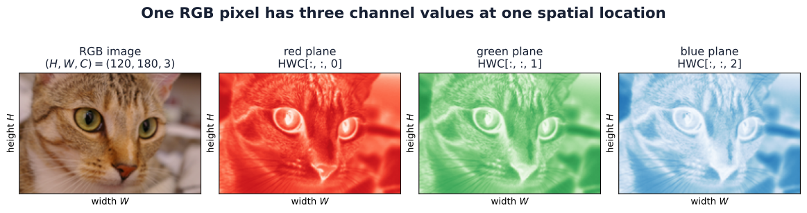
A color photograph of Chelsea the cat appears beside its red, green, and blue intensity planes, each labeled by its HWC channel index.
Figure 2: A color photograph of Chelsea the cat appears beside its red, green, and blue intensity planes, each labeled by its HWC channel index.

Interpretation. Height and width locate a pixel; the channel axis stores several measurements at that location. PyTorch puts the channel axis before the spatial axes and the batch axis before everything else.

Scene 2 — Fixed kernels: from one window to three response maps

Question. How can a small matrix ask the same local question everywhere in an image—and how does that calculation become F.conv2d?

We begin with a deliberately small \(7\times7\) image so every window and output location can be counted. Then we repeat the same operation on a genuine MNIST digit 3.

Three fixed local questions

Each \(3\times3\) kernel assigns weights to relative positions inside a local window:

  • blur averages the nine values;
  • horizontal edge compares the bottom row with the top row;
  • vertical edge compares the right column with the left column.

The sign carries orientation. With the kernels below, a horizontal response is positive for a dark-to-bright transition moving downward, and a vertical response is positive for a dark-to-bright transition moving rightward. Reversing the transition reverses the sign.

KERNELS = {
    "blur": torch.ones((3, 3), dtype=torch.float32) / 9,
    "horizontal edge": torch.tensor([[-1., -1., -1.],
                                      [ 0.,  0.,  0.],
                                      [ 1.,  1.,  1.]]),
    "vertical edge": torch.tensor([[-1., 0., 1.],
                                    [-1., 0., 1.],
                                    [-1., 0., 1.]]),
}
KERNEL_ORDER = ("blur", "horizontal edge", "vertical edge")
kernel_bank_hw = torch.stack([KERNELS[name] for name in KERNEL_ORDER])

# Student-editable control for the later MNIST scan.
KERNEL_NAME = "vertical edge"
assert KERNEL_NAME in KERNELS
selected_kernel_hw = KERNELS[KERNEL_NAME]

assert kernel_bank_hw.shape == (3, 3, 3)
for name, values in KERNELS.items():
    print(f"{name}:\n{values}\n")
print("kernel bank shape:", tuple(kernel_bank_hw.shape), "= (output channels, k_H, k_W)")
print(f'Selected later MNIST kernel: "{KERNEL_NAME}"')
blur:
tensor([[0.1111, 0.1111, 0.1111],
        [0.1111, 0.1111, 0.1111],
        [0.1111, 0.1111, 0.1111]])

horizontal edge:
tensor([[-1., -1., -1.],
        [ 0.,  0.,  0.],
        [ 1.,  1.,  1.]])

vertical edge:
tensor([[-1.,  0.,  1.],
        [-1.,  0.,  1.],
        [-1.,  0.,  1.]])

kernel bank shape: (3, 3, 3) = (output channels, k_H, k_W)
Selected later MNIST kernel: "vertical edge"

One window, three answers

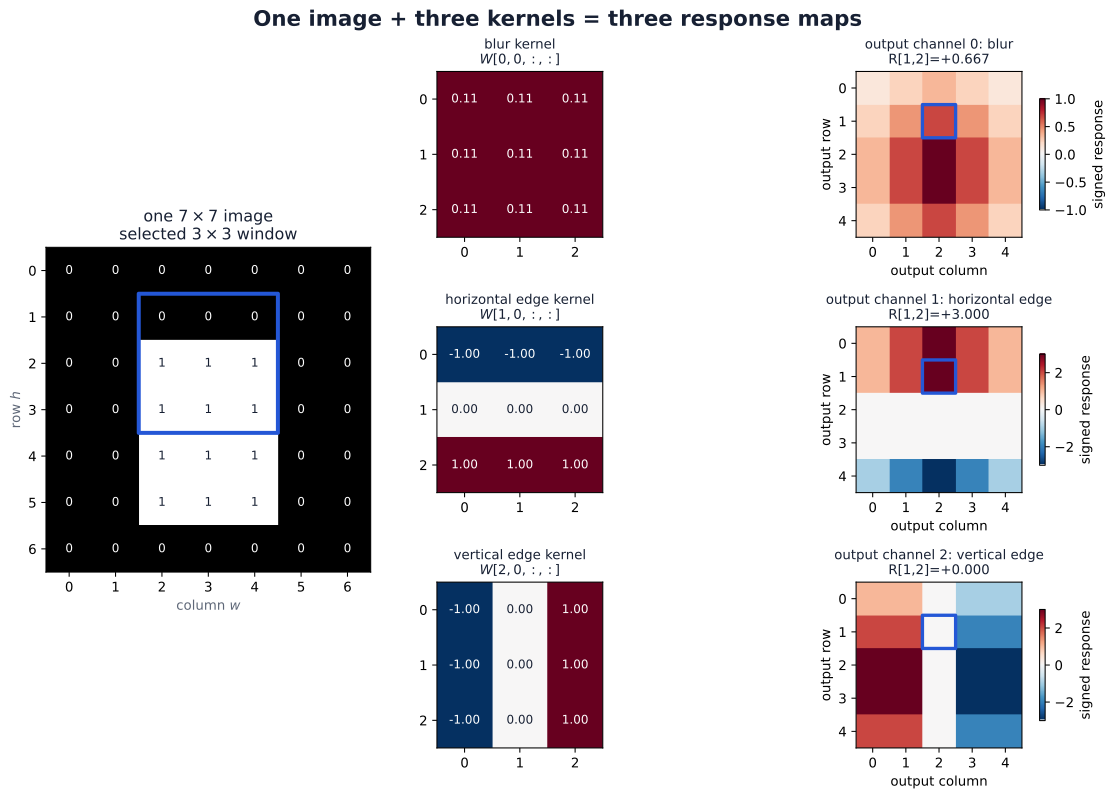
The small image contains one bright rectangle. Select the \(3\times3\) window beginning at zero-based location \((r,c)=(1,2)\). For each kernel, multiply matching entries and add all nine products:

\[ R^{(o)}_{r,c}=\sum_{u=0}^{2}\sum_{v=0}^{2} X_{r+u,c+v}\,W^{(o)}_{u,v}, \]

where \(o\) selects blur, horizontal edge, or vertical edge.

Prediction checkpoint. The selected window crosses the rectangle’s top boundary. Which kernel should have the largest positive response? Which edge response should cancel?

toy_image_hw = torch.zeros((7, 7), dtype=torch.float32)
toy_image_hw[2:6, 2:5] = 1.0
TOY_PATCH_ROW, TOY_PATCH_COLUMN = 1, 2
toy_patch_hw = toy_image_hw[
    TOY_PATCH_ROW:TOY_PATCH_ROW + 3,
    TOY_PATCH_COLUMN:TOY_PATCH_COLUMN + 3,
]
toy_products_ohw = kernel_bank_hw * toy_patch_hw.unsqueeze(0)
toy_hand_responses = toy_products_ohw.sum(dim=(1, 2))

assert toy_image_hw.shape == (7, 7)
assert toy_patch_hw.shape == (3, 3)
assert toy_products_ohw.shape == (3, 3, 3)
torch.testing.assert_close(
    toy_hand_responses, torch.tensor([6 / 9, 3.0, 0.0]),
    rtol=1e-6, atol=1e-6,
)
print("selected patch:\n", toy_patch_hw)
for name, products, response in zip(KERNEL_ORDER, toy_products_ohw, toy_hand_responses):
    print(f"\n{name}: products\n{products}\nsum = {response.item():+.3f}")
selected patch:
 tensor([[0., 0., 0.],
        [1., 1., 1.],
        [1., 1., 1.]])

blur: products
tensor([[0.0000, 0.0000, 0.0000],
        [0.1111, 0.1111, 0.1111],
        [0.1111, 0.1111, 0.1111]])
sum = +0.667

horizontal edge: products
tensor([[-0., -0., -0.],
        [0., 0., 0.],
        [1., 1., 1.]])
sum = +3.000

vertical edge: products
tensor([[-0.,  0.,  0.],
        [-1.,  0.,  1.],
        [-1.,  0.,  1.]])
sum = +0.000

The horizontal-edge kernel returns \(+3\): its negative top row meets zeros, while its positive bottom row meets three ones. The vertical-edge response is \(0\) because its left and right evidence balance. The blur returns \(6/9\) because six of the nine values are bright.

Slide the same weights across every valid window

A \(3\times3\) window has five valid row starts and five valid column starts in a \(7\times7\) image. Scanning therefore produces a \(5\times5\) response map for each kernel. The loops below make that mapping explicit before PyTorch performs the same work in one call.

toy_manual_responses_chw = torch.empty((3, 5, 5), dtype=torch.float32)
for output_channel, kernel_hw in enumerate(kernel_bank_hw):
    for output_row in range(5):
        for output_column in range(5):
            window_hw = toy_image_hw[
                output_row:output_row + 3,
                output_column:output_column + 3,
            ]
            toy_manual_responses_chw[output_channel, output_row, output_column] = (
                window_hw * kernel_hw
            ).sum()

# PyTorch adds the batch and input-channel axes expected by conv2d.
toy_input_bchw = toy_image_hw.unsqueeze(0).unsqueeze(0)
toy_weights_oihw = kernel_bank_hw.unsqueeze(1)
toy_pytorch_bchw = F.conv2d(toy_input_bchw, toy_weights_oihw)

assert toy_input_bchw.shape == (1, 1, 7, 7)
assert toy_weights_oihw.shape == (3, 1, 3, 3)
assert toy_pytorch_bchw.shape == (1, 3, 5, 5)
torch.testing.assert_close(toy_pytorch_bchw[0], toy_manual_responses_chw)
torch.testing.assert_close(
    toy_pytorch_bchw[0, :, TOY_PATCH_ROW, TOY_PATCH_COLUMN],
    toy_hand_responses,
)
print("input:", tuple(toy_input_bchw.shape), "= (B, C_in, H, W)")
print("weights:", tuple(toy_weights_oihw.shape), "= (C_out, C_in, k_H, k_W)")
print("output:", tuple(toy_pytorch_bchw.shape), "= (B, C_out, H_out, W_out)")
print("all 75 manual window responses match F.conv2d")

export_three_kernel_bridge(
    toy_image_hw, KERNEL_ORDER, kernel_bank_hw,
    toy_pytorch_bchw[0], (TOY_PATCH_ROW, TOY_PATCH_COLUMN),
)
input: (1, 1, 7, 7) = (B, C_in, H, W)
weights: (3, 1, 3, 3) = (C_out, C_in, k_H, k_W)
output: (1, 3, 5, 5) = (B, C_out, H_out, W_out)
all 75 manual window responses match F.conv2d
saved assets/figures/shared/week05/02-three-kernel-bridge.svg
saved assets/figures/shared/week05/02-three-kernel-bridge.png
(PosixPath('/Users/alexeykornaev/Documents/GitHub/Intro-to-ML-2026/assets/figures/shared/week05/02-three-kernel-bridge.svg'),
 PosixPath('/Users/alexeykornaev/Documents/GitHub/Intro-to-ML-2026/assets/figures/shared/week05/02-three-kernel-bridge.png'))
A seven-by-seven image with one selected three-by-three window feeds three rows. Each row shows a blur, horizontal-edge, or vertical-edge kernel and its complete five-by-five signed response map; the corresponding output cell is highlighted.
Figure 3: A seven-by-seven image with one selected three-by-three window feeds three rows. Each row shows a blur, horizontal-edge, or vertical-edge kernel and its complete five-by-five signed response map; the corresponding output cell is highlighted.

The bridge to PyTorch is entirely about axes:

  • the image changes from \((H,W)=(7,7)\) to input shape \((B,C_{\mathrm{in}},H,W)=(1,1,7,7)\);
  • the three stacked kernels change from \((3,3,3)\) to weight shape \((C_{\mathrm{out}},C_{\mathrm{in}},k_H,k_W)=(3,1,3,3)\);
  • F.conv2d returns \((B,C_{\mathrm{out}},H_{\mathrm{out}},W_{\mathrm{out}})=(1,3,5,5)\).

Thus one PyTorch output channel corresponds to one kernel and one complete response map. Such outputs are often informally called feature maps. Here the kernels are fixed, so response map is more precise; after the kernels are learned and an activation is applied, feature map or activation map becomes the natural term.

Apply one chosen kernel to a real digit

The tiny image made the mechanism countable. Now keep the same calculation and use the student-editable KERNEL_NAME on a genuine \(28\times28\) MNIST digit 3.

PyTorch stores this one-input-channel, one-output-channel kernel as \((C_{\mathrm{out}},C_{\mathrm{in}},k_H,k_W)=(1,1,3,3)\). With no bias, stride 1, and no padding, its fixed response at one location is

\[ R_{r,c}=\sum_{u=0}^{2}\sum_{v=0}^{2}X_{0,0,r+u,c+v}\,W_{0,0,u,v}. \]

This is the same indexed multiply-and-sum that will become \(z^{(\ell)}\) after trainable weights and a bias are introduced. No activation \(\phi\) is applied here, so call the result a response map, not an activation map.

digit_image_hw = torch.from_numpy(
    plt.imread(MEDIA_DIR / "mnist-train-00007-digit-3.png").copy()
).to(torch.float32)
digit_image_bchw = digit_image_hw.unsqueeze(0).unsqueeze(0)
selected_kernel_oihw = selected_kernel_hw.unsqueeze(0).unsqueeze(0)
H_in_digit, W_in_digit = digit_image_hw.shape
k_H_digit, k_W_digit = selected_kernel_hw.shape

# Chosen to cross a strong dark-to-bright vertical transition for the default kernel.
PATCH_ROW, PATCH_COLUMN = 16, 15
selected_digit_patch = digit_image_hw[
    PATCH_ROW:PATCH_ROW + k_H_digit,
    PATCH_COLUMN:PATCH_COLUMN + k_W_digit,
]

assert digit_image_bchw.shape == (1, 1, 28, 28)
assert selected_kernel_oihw.shape == (1, 1, 3, 3)
assert selected_digit_patch.shape == (3, 3)
assert torch.all((0 <= digit_image_hw) & (digit_image_hw <= 1))
print(f"input shape:  {tuple(digit_image_bchw.shape)} = (B, C_in, H_in, W_in)")
print(f"kernel shape: {tuple(selected_kernel_oihw.shape)} = (C_out, C_in, k_H, k_W)")
print("selected patch:\n", selected_digit_patch)
print(f'selected kernel "{KERNEL_NAME}":\n', selected_kernel_hw)
input shape:  (1, 1, 28, 28) = (B, C_in, H_in, W_in)
kernel shape: (1, 1, 3, 3) = (C_out, C_in, k_H, k_W)
selected patch:
 tensor([[0.1725, 0.5608, 0.9882],
        [0.0000, 0.0588, 0.9882],
        [0.0000, 0.3373, 0.9882]])
selected kernel "vertical edge":
 tensor([[-1.,  0.,  1.],
        [-1.,  0.,  1.],
        [-1.,  0.,  1.]])

Prediction checkpoint — one patch

Before running the next cell, inspect the patch and selected kernel. Predict the response’s sign and estimate its magnitude. Which columns will add positive evidence, and which will subtract evidence?

digit_products = selected_digit_patch * selected_kernel_hw
digit_hand_response = digit_products.sum()

assert digit_products.shape == (3, 3)
torch.testing.assert_close(
    digit_hand_response,
    sum(digit_products[u, v] for u in range(3) for v in range(3)),
    rtol=1e-6, atol=1e-6,
)
print("elementwise products:\n", digit_products)
print(f"R[{PATCH_ROW}, {PATCH_COLUMN}] = sum(products) = {digit_hand_response.item():+.6f}")
elementwise products:
 tensor([[-0.1725,  0.0000,  0.9882],
        [-0.0000,  0.0000,  0.9882],
        [-0.0000,  0.0000,  0.9882]])
R[16, 15] = sum(products) = +2.792157

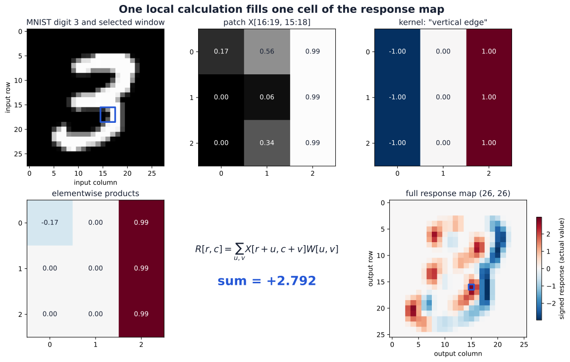
For the default vertical-edge kernel, the exact response is approximately \(+2.792157\). Bright values on the patch’s right side receive \(+1\) weights, while the left side contributes much less negative evidence. The stored kernel orientation fixes the sign.

Prediction checkpoint — the complete response map

For a valid scan with \((p_H,p_W)=(0,0)\) and \((s_H,s_W)=(1,1)\),

\[ H_{\mathrm{out}}=\left\lfloor\frac{H_{\mathrm{in}}-k_H}{1}\right\rfloor+1=26, \qquad W_{\mathrm{out}}=26. \]

Before scanning, predict which parts of the digit should give positive, negative, or near-zero responses for the selected kernel. Changing KERNEL_NAME should change that prediction before it changes the picture.

H_out_digit = H_in_digit - k_H_digit + 1
W_out_digit = W_in_digit - k_W_digit + 1
digit_response_hw = torch.empty((H_out_digit, W_out_digit), dtype=torch.float32)

for output_row in range(H_out_digit):
    for output_column in range(W_out_digit):
        patch = digit_image_hw[
            output_row:output_row + k_H_digit,
            output_column:output_column + k_W_digit,
        ]
        digit_response_hw[output_row, output_column] = (patch * selected_kernel_hw).sum()

assert digit_response_hw.shape == (26, 26)
torch.testing.assert_close(
    digit_response_hw[PATCH_ROW, PATCH_COLUMN], digit_hand_response, rtol=0, atol=0
)
print(f"response-map shape: {tuple(digit_response_hw.shape)} = (H_out, W_out)")
print(f"signed range: [{digit_response_hw.min().item():+.3f}, "
      f"{digit_response_hw.max().item():+.3f}]")
response-map shape: (26, 26) = (H_out, W_out)
signed range: [-2.969, +2.792]

Each loop iteration writes one local response to the output location with the same \((r,c)\) index. Signed values remain signed numbers; the visualization below uses a fixed zero-centered color scale and does not normalize the response map.

Check the entire scan against PyTorch

digit_response_bchw = F.conv2d(
    digit_image_bchw, selected_kernel_oihw, bias=None, stride=1, padding=0
)
assert digit_response_bchw.shape == (1, 1, 26, 26)
torch.testing.assert_close(digit_response_bchw[0, 0], digit_response_hw, rtol=1e-6, atol=1e-6)
print(f"PyTorch output: {tuple(digit_response_bchw.shape)} = (B, C_out, H_out, W_out)")
print("all 676 explicit responses match conv2d within 1e-6 floating-point tolerance")
PyTorch output: (1, 1, 26, 26) = (B, C_out, H_out, W_out)
all 676 explicit responses match conv2d within 1e-6 floating-point tolerance

torch.nn.functional.conv2d performs cross-correlation: it uses the displayed kernel without flipping it. PyTorch and this tutorial follow the deep-learning convention of calling that operation convolution.

Static key frame

The selected kernel’s name and values stay beside the image. The selected patch, elementwise products, sum, and corresponding output cell make the local-to-global mapping readable even if the animation does not play.

export_digit_kernel_keyframe(
    digit_image_hw, selected_kernel_hw, digit_response_hw,
    PATCH_ROW, PATCH_COLUMN, KERNEL_NAME,
);
A genuine MNIST digit 3 has one three-by-three window outlined. Beside it are the selected patch, the named vertical-edge kernel, their elementwise products, the signed sum, and the complete zero-centered response map with the matching output cell outlined.
Figure 4: A genuine MNIST digit 3 has one three-by-three window outlined. Beside it are the selected patch, the named vertical-edge kernel, their elementwise products, the signed sum, and the complete zero-centered response map with the matching output cell outlined.

Interpretation. The kernel is unchanged as location changes. A positive response means the patch aligns with the selected orientation; a negative response means the reverse orientation; a small response means cancellation or weak local evidence. These are exact response values, not brightness scores rescaled to \([0,1]\).

Motion view — one representative scan row

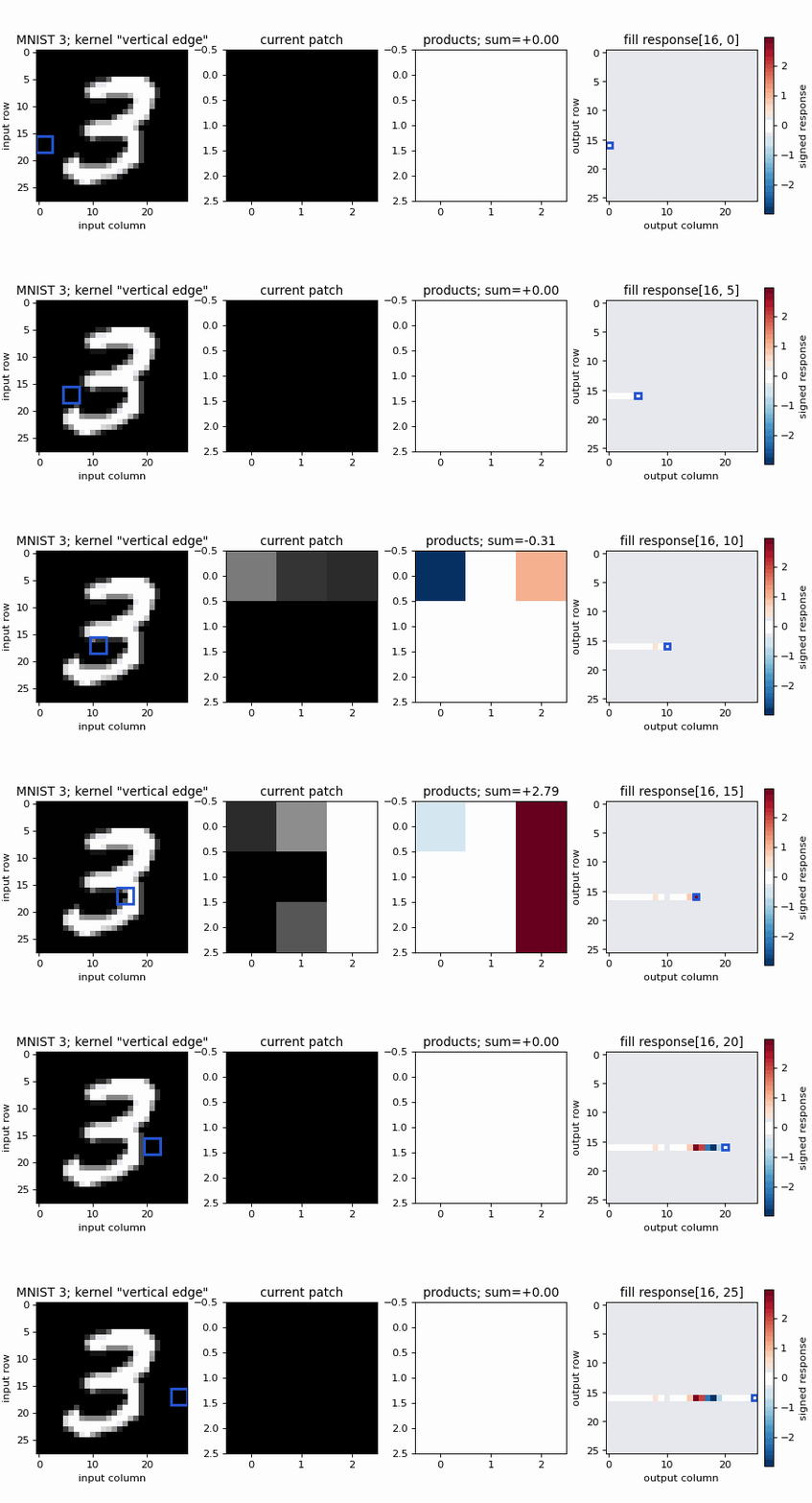
The compact animation follows all 26 valid windows in output row 16. It shows the current patch, products, sum, and output cell being filled. The static key frame above carries the complete explanation for slides, PDF, and environments where GIF playback is unavailable.

digit_animation_path = export_digit_scan_animation(
    digit_image_hw, selected_kernel_hw, digit_response_hw,
    scan_row=PATCH_ROW, kernel_name=KERNEL_NAME,
)
saved assets/figures/shared/week05/02-mnist3-convolution-scan.gif
animation frames: 26

A three-by-three window moves across one row of a genuine MNIST digit 3 while adjacent panels update the patch, elementwise products and sum, and the corresponding signed response-map cell.

A three-by-three window moves across one row of a genuine MNIST digit 3 while adjacent panels update the patch, elementwise products and sum, and the corresponding signed response-map cell.

Scene 3 — Trainable kernels: shared weights and shared gradients

Scene 2 used a fixed kernel to multiply each local window element by element and add the products. A convolutional layer performs the same local calculation, but its kernel entries are trainable entries of the layer parameter tensor \(\mathbf W^{(\ell)}\).

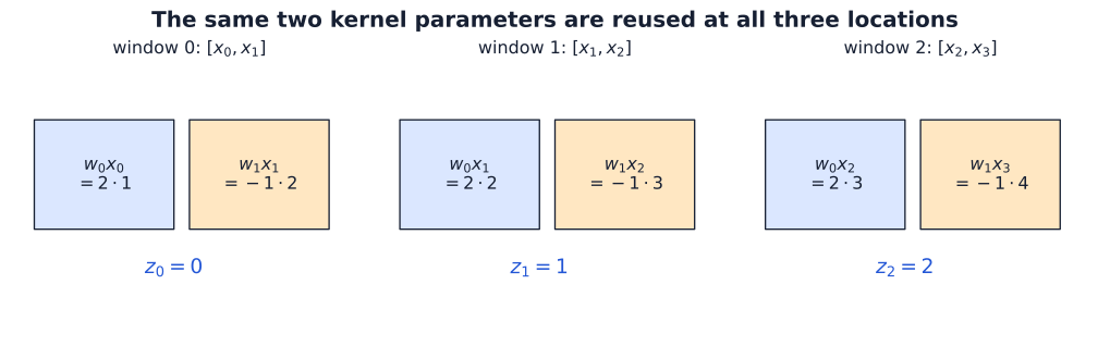
To see what sharing means, use one input channel, \(\mathbf x=[1,2,3,4]\), and a width-2 kernel \(\mathbf w=[w_0,w_1]=[2,-1]\). With no bias or activation, the three outputs are preactivations \(\mathbf z^{(\ell)}\).

Prediction checkpoint — reuse the same two parameters

Three overlapping width-2 windows fit in \(\mathbf x\). Before running the cell, predict \(z_0,z_1,z_2\). Which input value multiplies \(w_0\) and which multiplies \(w_1\) at each location? Why does this operation have two trainable parameters rather than six?

tiny_input = torch.tensor([1.0, 2.0, 3.0, 4.0])
tiny_kernel = torch.tensor([2.0, -1.0], requires_grad=True)
tiny_windows = tiny_input.unfold(dimension=0, size=2, step=1)

explicit_response = tiny_windows @ tiny_kernel
conv1d_response = F.conv1d(
    tiny_input.reshape(1, 1, 4), tiny_kernel.reshape(1, 1, 2)
).reshape(-1)

assert tiny_windows.shape == (3, 2)
assert tiny_kernel.shape == (2,)
torch.testing.assert_close(explicit_response, torch.tensor([0.0, 1.0, 2.0]))
torch.testing.assert_close(conv1d_response, explicit_response)
print(f"windows:\n{tiny_windows}")
print("z_0 = 2(1) - 1(2) = 0")
print("z_1 = 2(2) - 1(3) = 1")
print("z_2 = 2(3) - 1(4) = 2")
windows:
tensor([[1., 2.],
        [2., 3.],
        [3., 4.]])
z_0 = 2(1) - 1(2) = 0
z_1 = 2(2) - 1(3) = 1
z_2 = 2(3) - 1(4) = 2

The next compact diagram labels the reused parameters in all three local calculations.

export_shared_kernel_windows(tiny_input, tiny_kernel.detach(), explicit_response.detach())
saved assets/figures/shared/week05/03-shared-kernel-windows.svg
saved assets/figures/shared/week05/03-shared-kernel-windows.png
(PosixPath('/Users/alexeykornaev/Documents/GitHub/Intro-to-ML-2026/assets/figures/shared/week05/03-shared-kernel-windows.svg'),
 PosixPath('/Users/alexeykornaev/Documents/GitHub/Intro-to-ML-2026/assets/figures/shared/week05/03-shared-kernel-windows.png'))
Three overlapping pairs from the input one, two, three, four are shown. Each pair uses the same blue w-zero and orange w-one boxes, producing outputs zero, one, and two.
Figure 5: Three overlapping pairs from the input one, two, three, four are shown. Each pair uses the same blue w-zero and orange w-one boxes, producing outputs zero, one, and two.

The locations reuse the same \(w_0\) and \(w_1\): there are two stored parameters and three applications of each, not six independently adjustable values.

Shared uses produce shared gradients

Define

\[ J=z_0+z_1+z_2. \]

\(J\) is a deliberately simple scalar for examining gradients; it is not a training loss. Because \(\partial J/\partial z_j=1\), each location contributes the input value paired with a shared weight. Before running the cell, predict the two sums.

w0_contributions = tiny_windows[:, 0]  # x_0, x_1, x_2
w1_contributions = tiny_windows[:, 1]  # x_1, x_2, x_3
hand_gradient = torch.stack((w0_contributions.sum(), w1_contributions.sum()))

objective_J = conv1d_response.sum()
objective_J.backward()

torch.testing.assert_close(objective_J.detach(), torch.tensor(3.0))
torch.testing.assert_close(hand_gradient, torch.tensor([6.0, 9.0]))
torch.testing.assert_close(tiny_kernel.grad, hand_gradient)
print("∂J/∂w_0 = x_0 + x_1 + x_2 = 1 + 2 + 3 = 6")
print("∂J/∂w_1 = x_1 + x_2 + x_3 = 2 + 3 + 4 = 9")
print(f"autograd: {tiny_kernel.grad.tolist()}")
∂J/∂w_0 = x_0 + x_1 + x_2 = 1 + 2 + 3 = 6
∂J/∂w_1 = x_1 + x_2 + x_3 = 2 + 3 + 4 = 9
autograd: [6.0, 9.0]

This is Week 04’s backpropagation rule in a shared-parameter setting: derivatives multiply along each path, and contributions add where the paths meet. Autograd therefore accumulates the three uses into the two entries of \(\nabla_{\mathbf W^{(\ell)}}J\); no new differentiation rule is needed.

Optional linear-algebra view

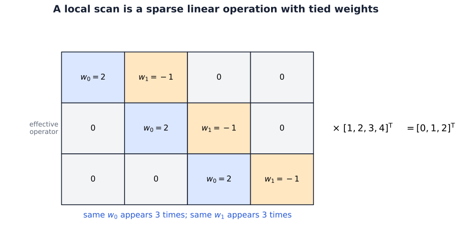
The same scan can be written as multiplication by a sparse matrix whose repeated labels are tied to the same parameters:

\[ \begin{bmatrix} w_0&w_1&0&0\\ 0&w_0&w_1&0\\ 0&0&w_0&w_1 \end{bmatrix}\mathbf x=\mathbf z. \]

zero = tiny_kernel.new_zeros(())
effective_matrix = torch.stack((
    torch.stack((tiny_kernel[0], tiny_kernel[1], zero, zero)),
    torch.stack((zero, tiny_kernel[0], tiny_kernel[1], zero)),
    torch.stack((zero, zero, tiny_kernel[0], tiny_kernel[1])),
))
matrix_response = effective_matrix @ tiny_input

assert effective_matrix.shape == (3, 4)
torch.testing.assert_close(matrix_response, conv1d_response.detach())
print(effective_matrix.detach())
print(f"matrix view response: {matrix_response.detach().tolist()}")
tensor([[ 2., -1.,  0.,  0.],
        [ 0.,  2., -1.,  0.],
        [ 0.,  0.,  2., -1.]])
matrix view response: [0.0, 1.0, 2.0]

The figure makes the repeated parameter identities in that optional matrix view explicit; its colours identify identity, not sign or magnitude.

export_shared_weights_sparse_operator(
    tiny_input, tiny_kernel.detach(), matrix_response.detach()
)
saved assets/figures/shared/week05/03-shared-weights-sparse-operator.svg
saved assets/figures/shared/week05/03-shared-weights-sparse-operator.png
(PosixPath('/Users/alexeykornaev/Documents/GitHub/Intro-to-ML-2026/assets/figures/shared/week05/03-shared-weights-sparse-operator.svg'),
 PosixPath('/Users/alexeykornaev/Documents/GitHub/Intro-to-ML-2026/assets/figures/shared/week05/03-shared-weights-sparse-operator.png'))
A three-by-four sparse matrix contains three diagonally shifted copies of two coloured labels, w-zero equals two and w-one equals negative one. It multiplies the four-value input to produce three responses; a note states that each labelled parameter appears three times.
Figure 6: A three-by-four sparse matrix contains three diagonally shifted copies of two coloured labels, w-zero equals two and w-one equals negative one. It multiplies the four-value input to produce three responses; a note states that each labelled parameter appears three times.

This matrix represents the local operation for analysis; Conv1d stores the width-2 kernel, not this expanded \(3\times4\) matrix.

Scene 4 — Color convolution: how does one filter combine RGB evidence?

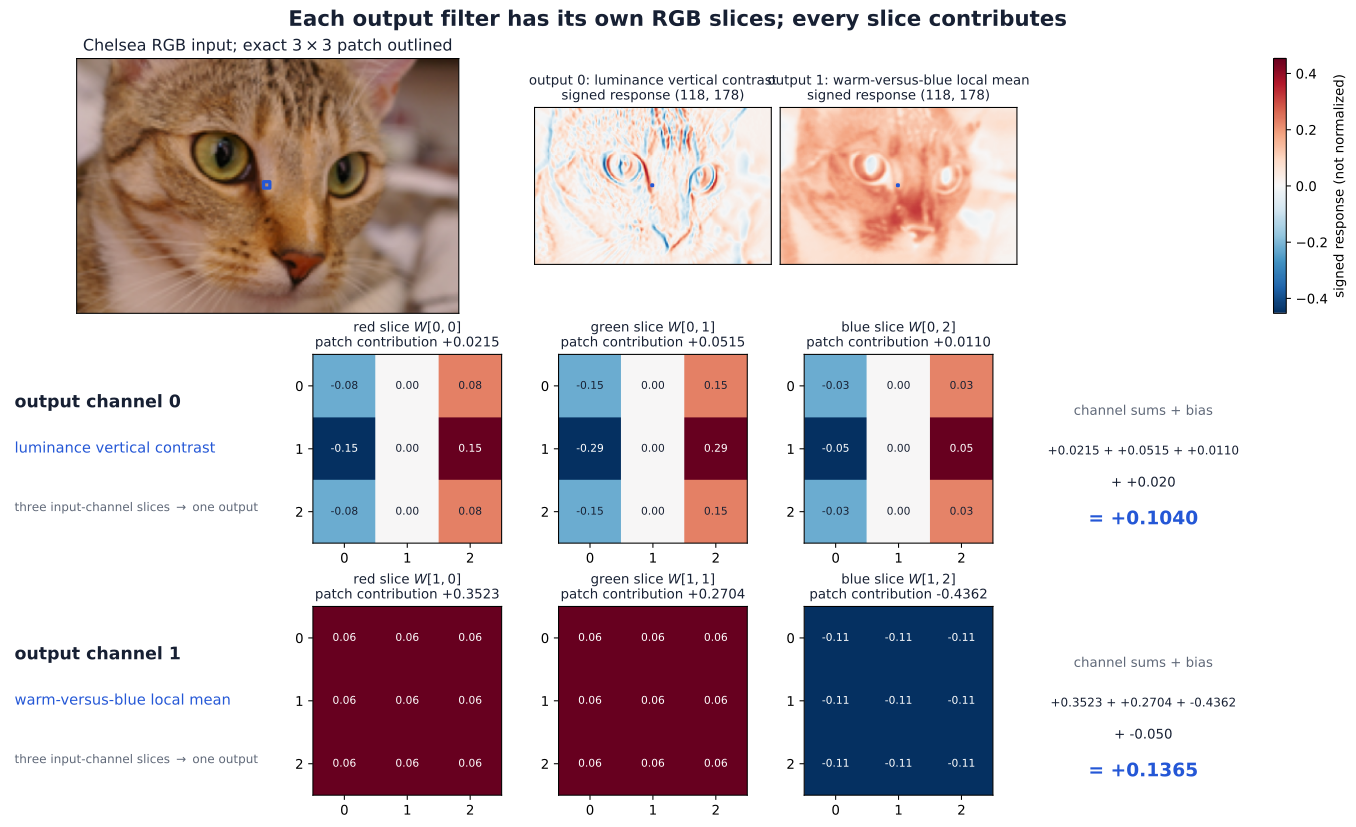
An RGB output is not produced by convolving the channels independently and keeping three answers. Each output channel owns one slice for every input channel, sums all three spatial contributions, and adds its own bias.

We will use two named \(3\times3\) filters on the full Chelsea image:

  • luminance vertical contrast applies the same vertical-edge geometry to red, green, and blue, weighted by approximate luminance importance;
  • warm-versus-blue local mean compares local red-and-green evidence with local blue evidence.

Both filters use all three input channels. They are hand-designed teaching filters, not learned features.

RGB_PATCH_ROW, RGB_PATCH_COLUMN = 58, 88
vertical_contrast = torch.tensor(
    [[-1.0, 0.0, 1.0], [-2.0, 0.0, 2.0], [-1.0, 0.0, 1.0]]
) / 4.0
local_mean = torch.ones((3, 3)) / 9.0
color_weight_oihw = torch.stack((
    torch.stack((0.30 * vertical_contrast,
                 0.59 * vertical_contrast,
                 0.11 * vertical_contrast)),
    torch.stack((0.50 * local_mean,
                 0.50 * local_mean,
                -1.00 * local_mean)),
))
color_bias = torch.tensor([0.02, -0.05])
COLOR_FILTER_NAMES = ("luminance vertical contrast", "warm-versus-blue local mean")

rgb_local_patches = rgb_photo_chw[
    :, RGB_PATCH_ROW:RGB_PATCH_ROW + 3, RGB_PATCH_COLUMN:RGB_PATCH_COLUMN + 3
]
assert rgb_local_patches.shape == (3, 3, 3)
assert color_weight_oihw.shape == (2, 3, 3, 3)
assert torch.all(color_weight_oihw.abs().sum(dim=(2, 3)) > 0)
print("RGB patch shape (C_in, k_H, k_W):", tuple(rgb_local_patches.shape))
print("weights (C_out, C_in, k_H, k_W):", tuple(color_weight_oihw.shape))
print("named output filters:", COLOR_FILTER_NAMES)
RGB patch shape (C_in, k_H, k_W): (3, 3, 3)
weights (C_out, C_in, k_H, k_W): (2, 3, 3, 3)
named output filters: ('luminance vertical contrast', 'warm-versus-blue local mean')

Prediction checkpoint — three contributions, then one output

For each named output filter, inspect its red, green, and blue slices. Predict which channel contributes most strongly at the outlined patch and whether the bias raises or lowers the cross-channel sum.

color_products = rgb_local_patches.unsqueeze(0) * color_weight_oihw
color_contributions = color_products.sum(dim=(2, 3))
color_hand_outputs = color_contributions.sum(dim=1) + color_bias

assert color_products.shape == (2, 3, 3, 3)
assert color_contributions.shape == (2, 3)
for output_channel, filter_name in enumerate(COLOR_FILTER_NAMES):
    print(f"{filter_name}:")
    for channel_name, value in zip(("red", "green", "blue"), color_contributions[output_channel]):
        print(f"  {channel_name:5s} contribution {value.item():+.6f}")
    print(f"  sum + bias {color_bias[output_channel].item():+.2f} "
          f"= {color_hand_outputs[output_channel].item():+.6f}")
luminance vertical contrast:
  red   contribution +0.021471
  green contribution +0.051480
  blue  contribution +0.011000
  sum + bias +0.02 = +0.103951
warm-versus-blue local mean:
  red   contribution +0.352288
  green contribution +0.270370
  blue  contribution -0.436166
  sum + bias -0.05 = +0.136492

The first output uses three edge-shaped slices with different channel weights. The second owns a different complete RGB filter. The numerical responses stay signed; later display colors are centered at zero but do not change the values.

color_output_bchw = F.conv2d(rgb_photo_bchw, color_weight_oihw, bias=color_bias)
assert color_output_bchw.shape == (1, 2, 118, 178)
torch.testing.assert_close(
    color_output_bchw[0, :, RGB_PATCH_ROW, RGB_PATCH_COLUMN],
    color_hand_outputs,
    rtol=1e-5, atol=1e-6,
)
print("full-image output shape (B, C_out, H_out, W_out):", tuple(color_output_bchw.shape))
print("both hand calculations match F.conv2d at the selected location")

export_color_convolution_keyframe(
    rgb_photo_hwc, (RGB_PATCH_ROW, RGB_PATCH_COLUMN), color_weight_oihw,
    color_bias, color_contributions, color_hand_outputs,
    color_output_bchw[0].detach(), COLOR_FILTER_NAMES,
)
full-image output shape (B, C_out, H_out, W_out): (1, 2, 118, 178)
both hand calculations match F.conv2d at the selected location
saved assets/figures/shared/week05/04-color-convolution-key-frame.svg
saved assets/figures/shared/week05/04-color-convolution-key-frame.png
(PosixPath('/Users/alexeykornaev/Documents/GitHub/Intro-to-ML-2026/assets/figures/shared/week05/04-color-convolution-key-frame.svg'),
 PosixPath('/Users/alexeykornaev/Documents/GitHub/Intro-to-ML-2026/assets/figures/shared/week05/04-color-convolution-key-frame.png'))
The Chelsea RGB image and two signed response maps appear above two filter rows. Each row shows that output channel's red, green, and blue kernel slices, the three exact patch contributions, their sum, bias, and selected output value.
Figure 7: The Chelsea RGB image and two signed response maps appear above two filter rows. Each row shows that output channel’s red, green, and blue kernel slices, the three exact patch contributions, their sum, bias, and selected output value.

The full image makes the names testable: one map responds to vertical luminance changes, while the other is high where a local patch is warmer than its blue channel. They are not semantic detectors, and their signed values are not display-normalized measurements.

Only now do we need the indexed rule:

\[ z^{(\ell)}_{b,o,r,c}=b^{(\ell)}_o+ \sum_{i=0}^{C_{\mathrm{in}}-1}\sum_{u=0}^{k_H-1}\sum_{v=0}^{k_W-1} W^{(\ell)}_{o,i,u,v}\, h^{(\ell-1)}_{b,i,\,r s_H+u-p_H,\,c s_W+v-p_W}. \]

PyTorch stores the weights in \((C_{\mathrm{out}},C_{\mathrm{in}},k_H,k_W)\) order. Here that is \((2,3,3,3)\): two independently parameterized output filters, each with three input-channel slices.

assert color_weight_oihw.numel() == 54
assert color_bias.numel() == 2
assert color_output_bchw.shape == (1, 2, 118, 178)
print("parameters: 2*3*3*3 weights + 2 biases = 56")
print("selected outputs:", color_output_bchw[0, :, RGB_PATCH_ROW, RGB_PATCH_COLUMN].tolist())
parameters: 2*3*3*3 weights + 2 biases = 56
selected outputs: [0.10395099222660065, 0.13649244606494904]

Scene 5 — Spatial controls: padding, stride, pooling, and receptive fields

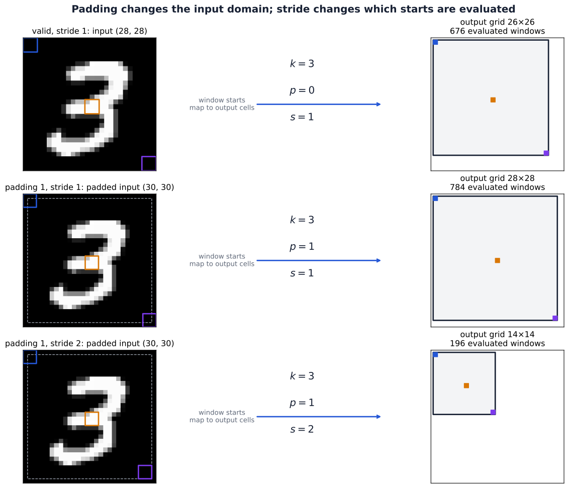
Use the real MNIST digit and the named "vertical edge" kernel from Scene 2. Padding and stride control where the kernel is evaluated. Pooling is a later, separate operation on the resulting map.

For dilation 1, the spatial output sizes are

\[ H_{\mathrm{out}}=\left\lfloor\frac{H_{\mathrm{in}}+2p_H-k_H}{s_H}\right\rfloor+1, \qquad W_{\mathrm{out}}=\left\lfloor\frac{W_{\mathrm{in}}+2p_W-k_W}{s_W}\right\rfloor+1. \]

Step 1 — valid scan, stride 1

Prediction checkpoint: with input \((28,28)\), kernel \((3,3)\), padding \((0,0)\), and stride \((1,1)\), predict the output shape and the first, middle, and last window starts.

def local_output_size(input_size, kernel_size, padding, stride):
    return (input_size + 2 * padding - kernel_size) // stride + 1

spatial_kernel_name = "vertical edge"
spatial_kernel_hw = KERNELS[spatial_kernel_name]
spatial_kernel_oihw = spatial_kernel_hw.reshape(1, 1, 3, 3)
valid_digit_hw = F.conv2d(digit_image_bchw, spatial_kernel_oihw, padding=0, stride=1)[0, 0]
valid_shape = tuple(valid_digit_hw.shape)

assert valid_shape == (26, 26)
assert valid_shape == tuple(local_output_size(28, 3, 0, 1) for _ in range(2))
valid_examples = [(0, 0), (13, 13), (25, 25)]
print("valid p=(0,0), s=(1,1):", valid_shape, "example starts:", valid_examples)
valid p=(0,0), s=(1,1): (26, 26) example starts: [(0, 0), (13, 13), (25, 25)]

Step 2 — zero padding 1, stride 1

Prediction checkpoint: adding one zero on every side changes the effective spatial input to \((30,30)\). Predict the output shape. In padded coordinates, output \((r,c)\) starts at \((r,c)\); relative to the original digit, that start is \((r-1,c-1)\).

padded_s1_digit_hw = F.conv2d(digit_image_bchw, spatial_kernel_oihw, padding=1, stride=1)[0, 0]
explicit_padded_digit = F.pad(digit_image_bchw, (1, 1, 1, 1))
explicit_padded_s1 = F.conv2d(explicit_padded_digit, spatial_kernel_oihw, stride=1)[0, 0]

assert explicit_padded_digit.shape == (1, 1, 30, 30)
assert padded_s1_digit_hw.shape == (28, 28)
torch.testing.assert_close(padded_s1_digit_hw, explicit_padded_s1, rtol=0, atol=0)
padded_s1_examples = [(0, 0), (14, 14), (27, 27)]
print("padding p=(1,1), s=(1,1):", tuple(padded_s1_digit_hw.shape))
print("padded starts:", padded_s1_examples, "; original-coordinate starts: [(-1,-1), (13,13), (26,26)]")
padding p=(1,1), s=(1,1): (28, 28)
padded starts: [(0, 0), (14, 14), (27, 27)] ; original-coordinate starts: [(-1,-1), (13,13), (26,26)]

Step 3 — zero padding 1, stride 2

Prediction checkpoint: stride 2 keeps every second padded-input start. Predict the output shape and the padded-coordinate starts for the first, middle, and last examples.

padded_s2_digit_hw = F.conv2d(digit_image_bchw, spatial_kernel_oihw, padding=1, stride=2)[0, 0]
assert padded_s2_digit_hw.shape == (14, 14)
assert tuple(padded_s2_digit_hw.shape) == tuple(local_output_size(28, 3, 1, 2) for _ in range(2))
padded_s2_examples = [(0, 0), (7, 7), (13, 13)]
padded_s2_starts = [(2 * r, 2 * c) for r, c in padded_s2_examples]
assert padded_s2_starts == [(0, 0), (14, 14), (26, 26)]
print("padding p=(1,1), s=(2,2):", tuple(padded_s2_digit_hw.shape))
print("example padded-input starts:", padded_s2_starts)
padding p=(1,1), s=(2,2): (14, 14)
example padded-input starts: [(0, 0), (14, 14), (26, 26)]

The three cases use the same signed kernel values. Padding adds boundary locations; stride changes the spacing of evaluated windows. Neither silently rescales the numerical responses.

Step 4 — \(2\times2\) max pooling

Name the padded stride-1 response map pool_source_hw. A \(2\times2\) max pool with stride 2 keeps the largest signed response in each non-overlapping window. It summarizes local evidence and loses the other three values; it does not guarantee invariance.

Prediction checkpoint: for the selected window feeding pooled output \((8,8)\), identify which of its four response values should win before running the cell.

pool_source_hw = padded_s1_digit_hw
max_pooled_digit_hw = F.max_pool2d(pool_source_hw.reshape(1, 1, 28, 28), 2, stride=2)[0, 0]
POOL_OUTPUT_INDEX = (8, 8)
pool_row, pool_column = (2 * POOL_OUTPUT_INDEX[0], 2 * POOL_OUTPUT_INDEX[1])
selected_pool_window = pool_source_hw[pool_row:pool_row + 2, pool_column:pool_column + 2]
selected_pool_winner = selected_pool_window.max()
winner_offset = tuple(int(v) for v in torch.nonzero(selected_pool_window == selected_pool_winner)[0])

assert selected_pool_window.shape == (2, 2)
assert max_pooled_digit_hw.shape == (14, 14)
torch.testing.assert_close(max_pooled_digit_hw[POOL_OUTPUT_INDEX], selected_pool_winner)
print("selected response window:\n", selected_pool_window)
print("winner offset within window:", winner_offset)
print("winner value:", selected_pool_winner.item())
print("pooled shape:", tuple(max_pooled_digit_hw.shape))
selected response window:
 tensor([[1.8039, 1.3569],
        [2.7922, 2.0078]])
winner offset within window: (1, 0)
winner value: 2.79215669631958
pooled shape: (14, 14)

The figure below connects each highlighted input-window start to one output cell. All three rows use the same \(3\times3\) kernel; only padding and stride change.

spatial_cases = [
    ("valid, stride 1", valid_digit_hw, 0, 1, [(0, 0), (13, 13), (25, 25)]),
    ("padding 1, stride 1", padded_s1_digit_hw, 1, 1, [(0, 0), (14, 14), (27, 27)]),
    ("padding 1, stride 2", padded_s2_digit_hw, 1, 2, [(0, 0), (14, 14), (26, 26)]),
]
export_spatial_controls_keyframes(digit_image_hw, spatial_kernel_hw, spatial_cases)
saved assets/figures/shared/week05/05-spatial-controls-key-frames.svg
saved assets/figures/shared/week05/05-spatial-controls-key-frames.png
(PosixPath('/Users/alexeykornaev/Documents/GitHub/Intro-to-ML-2026/assets/figures/shared/week05/05-spatial-controls-key-frames.svg'),
 PosixPath('/Users/alexeykornaev/Documents/GitHub/Intro-to-ML-2026/assets/figures/shared/week05/05-spatial-controls-key-frames.png'))
Three rows connect an input or explicitly padded input to its output grid. Colored three-by-three windows mark first, middle, and last starts; parameter boxes list kernel, padding, and stride; matching colored output cells show the different grid sizes.
Figure 8: Three rows connect an input or explicitly padded input to its output grid. Colored three-by-three windows mark first, middle, and last starts; parameter boxes list kernel, padding, and stride; matching colored output cells show the different grid sizes.

Valid scanning omits starts that would cross the boundary. Padding creates a larger input domain, restoring a \(28\times28\) output at stride 1. Stride 2 evaluates every second padded start, so the output has only \(14\times14\) cells.

Max pooling — four values become one

The earlier calculation selected the \(2\times2\) response window feeding pooled output \((8,8)\). The next figure shows the value-selection rule directly.

export_pooling_window(
    selected_pool_window, selected_pool_winner, winner_offset, POOL_OUTPUT_INDEX
)

layer_specs = [(3, 1), (2, 2)]
receptive_field_size, output_spacing = 1, 1
receptive_field_ledger = []
for layer_number, (kernel_width, stride) in enumerate(layer_specs, start=1):
    receptive_field_size += (kernel_width - 1) * output_spacing
    output_spacing *= stride
    receptive_field_ledger.append((layer_number, receptive_field_size, output_spacing))

def trace_input_coordinates(output_index, specs):
    coordinates = {output_index}
    for kernel_width, stride in reversed(specs):
        coordinates = {coordinate * stride + offset
                       for coordinate in coordinates for offset in range(kernel_width)}
    return sorted(coordinates)

traced_coordinates = {index: trace_input_coordinates(index, layer_specs) for index in range(3)}
assert receptive_field_ledger == [(1, 3, 1), (2, 4, 2)]
assert traced_coordinates == {0: [0, 1, 2, 3], 1: [2, 3, 4, 5], 2: [4, 5, 6, 7]}
assert receptive_field_size == 4 and output_spacing == 2
print("ledger (layer, receptive-field size, spacing):", receptive_field_ledger)
print("input coordinates:", traced_coordinates)
saved assets/figures/shared/week05/05-max-pooling-window.svg
saved assets/figures/shared/week05/05-max-pooling-window.png
ledger (layer, receptive-field size, spacing): [(1, 3, 1), (2, 4, 2)]
input coordinates: {0: [0, 1, 2, 3], 1: [2, 3, 4, 5], 2: [4, 5, 6, 7]}

The receptive-field size is 4, while adjacent layer-2 outputs are spaced 2 input coordinates apart. The diagram exposes the missing middle step: each layer-2 output first depends on two layer-1 values, and each of those depends on three input values. Overlap makes the union four inputs wide, not six.

export_receptive_field_trace(traced_coordinates, receptive_field_size, output_spacing)
saved assets/figures/shared/week05/05-receptive-field-trace.svg
saved assets/figures/shared/week05/05-receptive-field-trace.png
(PosixPath('/Users/alexeykornaev/Documents/GitHub/Intro-to-ML-2026/assets/figures/shared/week05/05-receptive-field-trace.svg'),
 PosixPath('/Users/alexeykornaev/Documents/GitHub/Intro-to-ML-2026/assets/figures/shared/week05/05-receptive-field-trace.png'))
A three-level dependency graph shows input positions, width-three stride-one layer-1 units, and two adjacent width-two stride-two layer-2 units. Their paths end in overlapping four-position input regions whose starts are two positions apart.
Figure 9: A three-level dependency graph shows input positions, width-three stride-one layer-1 units, and two adjacent width-two stride-two layer-2 units. Their paths end in overlapping four-position input regions whose starts are two positions apart.

Scene 6 — Our first 2D CNN

The earlier scenes isolated individual convolutional operations. Now combine them into a compact classifier for an explicit batch-first grayscale input \((B,1,28,28)\). We reuse the checked-in MNIST digit for one forward pass; no 2D dataset is downloaded or trained.

The model follows a short path:

\[ \text{Conv2d}\rightarrow\text{ReLU}\rightarrow\text{max pool} \rightarrow\text{Conv2d}\rightarrow\text{ReLU}\rightarrow\text{global average pool} \rightarrow\text{class logits}. \]

class TinyImageCNN(nn.Module):
    def __init__(self, number_of_classes=10):
        super().__init__()
        self.conv1 = nn.Conv2d(1, 8, kernel_size=3, padding=1)
        self.pool = nn.MaxPool2d(kernel_size=2, stride=2)
        self.conv2 = nn.Conv2d(8, 16, kernel_size=3, padding=1)
        self.global_pool = nn.AdaptiveAvgPool2d((1, 1))
        self.classifier = nn.Linear(16, number_of_classes)

    def forward(self, x):
        h1 = F.relu(self.conv1(x))
        h1_pooled = self.pool(h1)
        h2 = F.relu(self.conv2(h1_pooled))
        pooled = self.global_pool(h2)
        return self.classifier(pooled.flatten(1))


torch.manual_seed(202606)
tiny_image_cnn = TinyImageCNN(number_of_classes=10)
image_batch = digit_image_bchw
assert image_batch.shape == (1, 1, 28, 28)

Checked shape and parameter ledger

Predict each spatial shape before revealing the ledger. Padding 1 keeps each convolution’s height and width; the \(2\times2\) stride-2 pool halves both spatial axes. Global average pooling then replaces each \(14\times14\) channel map by one number.

with torch.no_grad():
    cnn_h1 = F.relu(tiny_image_cnn.conv1(image_batch))
    cnn_h1_pooled = tiny_image_cnn.pool(cnn_h1)
    cnn_h2 = F.relu(tiny_image_cnn.conv2(cnn_h1_pooled))
    cnn_global = tiny_image_cnn.global_pool(cnn_h2)
    cnn_logits = tiny_image_cnn.classifier(cnn_global.flatten(1))

cnn_ledger = [
    ("input", tuple(image_batch.shape), 0),
    ("conv1", tuple(cnn_h1.shape), 80),
    ("ReLU", tuple(cnn_h1.shape), 0),
    ("max pool", tuple(cnn_h1_pooled.shape), 0),
    ("conv2", tuple(cnn_h2.shape), 1168),
    ("ReLU", tuple(cnn_h2.shape), 0),
    ("global avg pool", tuple(cnn_global.shape), 0),
    ("flatten", (1, 16), 0),
    ("class logits", tuple(cnn_logits.shape), 170),
]

assert cnn_h1.shape == (1, 8, 28, 28)
assert cnn_h1_pooled.shape == (1, 8, 14, 14)
assert cnn_h2.shape == (1, 16, 14, 14)
assert cnn_global.shape == (1, 16, 1, 1)
assert cnn_logits.shape == (1, 10)
assert tiny_image_cnn.conv1.weight.shape == (8, 1, 3, 3)
assert tiny_image_cnn.conv2.weight.shape == (16, 8, 3, 3)
assert sum(parameter.numel() for parameter in tiny_image_cnn.parameters()) == 1418

print("stage                 output shape          trainable parameters")
for name, shape, parameters in cnn_ledger:
    print(f"{name:21s} {str(shape):21s} {parameters:>7d}")
print("total trainable parameters: 1418")
stage                 output shape          trainable parameters
input                 (1, 1, 28, 28)              0
conv1                 (1, 8, 28, 28)             80
ReLU                  (1, 8, 28, 28)              0
max pool              (1, 8, 14, 14)              0
conv2                 (1, 16, 14, 14)          1168
ReLU                  (1, 16, 14, 14)             0
global avg pool       (1, 16, 1, 1)               0
flatten               (1, 16)                     0
class logits          (1, 10)                   170
total trainable parameters: 1418

The first convolution has \(8(1\cdot3\cdot3+1)=80\) parameters. For a like-for-like connectivity comparison, define a dense layer that maps the flattened 784-pixel input to all \(8\cdot28\cdot28=6{,}272\) first-stage outputs. That dense alternative would require \(6{,}272(784+1)=4{,}923{,}520\) parameters. The comparison holds the output count fixed; the difference is local shared connectivity versus an independent weight from every pixel to every output.

conv1_parameters = tiny_image_cnn.conv1.weight.numel() + tiny_image_cnn.conv1.bias.numel()
dense_first_stage_outputs = 8 * 28 * 28
dense_alternative_parameters = dense_first_stage_outputs * (28 * 28 + 1)
assert conv1_parameters == 80
assert dense_first_stage_outputs == 6272
assert dense_alternative_parameters == 4_923_520
print(f"first Conv2d: {conv1_parameters:,} parameters")
print(f"dense 784-to-6272 alternative: {dense_alternative_parameters:,} parameters")
first Conv2d: 80 parameters
dense 784-to-6272 alternative: 4,923,520 parameters

The following figure records the architecture rather than random activation maps. A forward pass can verify tensor shapes and parameter counts, but the randomly initialized model has not supplied evidence that any channel detects a useful feature.

export_cnn_architecture(digit_image_hw, cnn_ledger)
saved assets/figures/shared/week05/06-cnn-architecture.svg
saved assets/figures/shared/week05/06-cnn-architecture.png
(PosixPath('/Users/alexeykornaev/Documents/GitHub/Intro-to-ML-2026/assets/figures/shared/week05/06-cnn-architecture.svg'),
 PosixPath('/Users/alexeykornaev/Documents/GitHub/Intro-to-ML-2026/assets/figures/shared/week05/06-cnn-architecture.png'))
A left-to-right structural diagram carries one grayscale input through Conv2d and ReLU, max pooling, a second Conv2d and ReLU, global average pooling, flattening, and a linear classifier. Every stage lists its tensor shape and parameter count.
Figure 10: A left-to-right structural diagram carries one grayscale input through Conv2d and ReLU, max pooling, a second Conv2d and ReLU, global average pooling, flattening, and a linear classifier. Every stage lists its tensor shape and parameter count.

What the checks establish. The code establishes that the architecture is internally consistent: every tensor has the predicted shape, the two convolutions and classifier account for 1,418 parameters, and the forward pass returns ten logits.

What training evidence would establish. Only optimization and held-out evaluation could show that those parameters learn useful detectors and support classification. Randomly initialized logits and shape checks cannot establish a feature hierarchy or predictive ability.

Scene 7 — Read two architecture papers

This scene is a guided reading, not an implementation. Consult the original AlexNet paper (Krizhevsky et al. 2012) and residual-learning paper (He et al. 2016).

AlexNet: paper report and Torchvision variant

The 2012 network has five convolutional and three fully connected learned layers. This reading aid records what Section 3.5 reports while collapsing the historical two-GPU partition into total channel counts. It deliberately omits exact spatial dimensions: the paper’s stated \(224\times224\) input, \(11\times11\) first kernel, stride 4, and \(55\times55\) first response require an additional boundary convention to reproduce together.

Stage What the original paper reports
conv1 96 kernels, \(11\times11\), stride 4; ReLU, response normalization, then \(3\times3\) max pooling with stride 2
conv2 256 kernels, \(5\times5\); ReLU, response normalization, then \(3\times3\) max pooling with stride 2
conv3–5 \(3\times3\) convolutions with 384, 384, then 256 channels; ReLU after each; pooling after conv5
classifier two 4096-unit fully connected layers, then a 1000-way output

The repeated pattern is convolutional processing followed by occasional spatial reduction. Channel counts generally rise as the spatial grid shrinks; most parameters reside in the globally connected part, not in the convolutional layers.

The graph below is not a literal reconstruction of the 2012 paper. It is an automatically traced, untrained Torchvision AlexNet variant, whose padding and implementation details give reproducible tensor shapes for a \(1\times3\times224\times224\) input.

Compact automatically traced overview of the untrained Torchvision AlexNet variant, listing convolution, pooling, adaptive-pooling, and fully connected stage shapes.

Compact automatically traced overview of the untrained Torchvision AlexNet variant, listing the convolution, pooling, adaptive-pooling, and fully connected stage shapes.

Open the complete Torchvision AlexNet variant graph as a zoomable SVG. It contains every traced operation, every learned layer, tensor shapes, parameter counts, and connections.

ResNet-18: residual blocks and two shortcut cases

The next overview is an automatically traced, untrained Torchvision ResNet-18 implementation of the architecture discussed in the residual-learning paper. It is an implementation view, not a copied paper figure.

Compact automatically traced overview of untrained Torchvision ResNet-18, from its stem through four residual stages, global average pooling, and class logits.

Compact automatically traced overview of untrained Torchvision ResNet-18, from its stem through four residual stages, global average pooling, and class logits.

Open the complete Torchvision ResNet-18 graph as a zoomable SVG. The complete graph retains all eight shortcut branches and their elementwise-addition nodes.

For matching input and output shapes, the residual paper defines

\[ \mathbf y = F(\mathbf x;\mathbf W)+\mathbf x. \]

The main branch learns the residual function \(F\). The identity path carries the exact block input \(\mathbf x\) around that branch; the two equally shaped tensors meet at an elementwise addition, not concatenation. The identity shortcut therefore adds no trainable parameters.

Automatically traced detail of ResNet-18 layer one block zero, with the input splitting into an unchanged identity shortcut and a two-convolution residual branch before elementwise addition.

Automatically traced detail of ResNet-18 layer 1 block 0, with the input splitting into an unchanged identity shortcut and a two-convolution residual branch before elementwise addition.

When spatial size or channel count changes, \(F(\mathbf x)\) and \(\mathbf x\) cannot be added directly. The paper describes a learned linear projection on the shortcut to match dimensions:

\[ \mathbf y = F(\mathbf x;\mathbf W)+W_s\mathbf x. \]

In Torchvision ResNet-18, the first block of layers 2–4 uses a \(1\times1\) projection convolution with stride 2, followed by batch normalization. The traced graph also contains BatchNorm2d throughout the residual branches and after the stem convolution. The Week 05 lecture will explain why normalization is used; this tutorial only asks you to recognize it in the architecture and does not implement it. This changes both the channel count and spatial size so the shortcut and residual branch have identical shapes at the addition.

Automatically traced detail of ResNet-18 layer two block zero, where both the residual branch and a projection shortcut reduce the spatial grid and produce 128 channels before elementwise addition.

Automatically traced detail of ResNet-18 layer 2 block 0, where both the residual branch and a projection shortcut reduce the spatial grid and produce 128 channels before elementwise addition.

Questions for the papers

  1. In AlexNet, after which convolutional stages does max pooling occur, and how do the spatial size and channel count change across those reductions?
  2. Why could the convolutional layers contain a small fraction of AlexNet’s parameters even though they dominate its spatial processing?
  3. In a residual block, what exact shape condition permits the identity shortcut, and what must the projection \(W_s\) change when that condition fails?

Core experiment — MLP versus Conv1d on MNIST-1D

Question. Does local connectivity and weight sharing change what a compact model learns from an ordered one-dimensional signal?

MNIST-1D is a synthetic dataset by Sam Greydanus and Dmitry Kobak. Class number \(0,1,\ldots,9\) names a generating template. The supplied examples are noisy, transformed length-40 waveforms—not flattened handwritten-MNIST images.

The official authors’ construction explanation at the pinned revision describes padding, translation, scaling, shear, correlated noise, and iid noise. We can illustrate these mechanisms, but we cannot recover the exact random transformation parameters of a displayed sample.

The unchanged train/test archive contains only x, y, x_test, and y_test. A second tiny safe archive stores the official frozen templates arrays for explanation. Both were converted once from the checksum-verified official pickle and load with allow_pickle=False; notebook execution makes no network request and loads no pickle.

MNIST1D_PATH = DATA_DIR / "mnist1d-official.npz"
TEMPLATE_PATH = DATA_DIR / "mnist1d-templates.npz"
EXPECTED_ARCHIVE_SHA256 = "ac56ec3c34fe9bdaf8f2d95cbb3831b3bd88d39f71968fe573cf055e0d237ecb"
EXPECTED_TEMPLATE_SHA256 = "15fa91e6eeef6964ed60431e35600d75388fadf442ada86ff07f641f4ef93c2e"
archive_sha256 = hashlib.sha256(MNIST1D_PATH.read_bytes()).hexdigest()
template_sha256 = hashlib.sha256(TEMPLATE_PATH.read_bytes()).hexdigest()
assert archive_sha256 == EXPECTED_ARCHIVE_SHA256
assert template_sha256 == EXPECTED_TEMPLATE_SHA256

with np.load(MNIST1D_PATH, allow_pickle=False) as archive:
    supplied_train_x = torch.from_numpy(archive["x"].copy()).to(torch.float32)
    supplied_train_y = torch.from_numpy(archive["y"].copy()).to(torch.long)
    supplied_test_x = torch.from_numpy(archive["x_test"].copy()).to(torch.float32)
    supplied_test_y = torch.from_numpy(archive["y_test"].copy()).to(torch.long)
with np.load(TEMPLATE_PATH, allow_pickle=False) as archive:
    template_x = torch.from_numpy(archive["x"].copy()).to(torch.float32)
    template_t = torch.from_numpy(archive["t"].copy()).to(torch.float32)
    template_y = torch.from_numpy(archive["y"].copy()).to(torch.long)

assert supplied_train_x.shape == (4000, 40)
assert supplied_test_x.shape == (1000, 40)
assert template_x.shape == (10, 12) and template_t.shape == (12,)
assert torch.equal(template_y, torch.arange(10))
print("official data archive SHA-256:", archive_sha256)
print("official template archive SHA-256:", template_sha256)
print("supplied train/test shapes:", tuple(supplied_train_x.shape), tuple(supplied_test_x.shape))
official data archive SHA-256: ac56ec3c34fe9bdaf8f2d95cbb3831b3bd88d39f71968fe573cf055e0d237ecb
official template archive SHA-256: 15fa91e6eeef6964ed60431e35600d75388fadf442ada86ff07f641f4ef93c2e
supplied train/test shapes: (4000, 40) (1000, 40)

What does a class label mean?

First inspect all ten clean source templates. Then hold the label fixed at class 3 and compare its template with three actual supplied training signals. The horizontal order matters in both, but the generated signals have length 40 after the data-generation pipeline.

export_mnist1d_templates_and_variation(
    template_x, template_t, template_y, supplied_train_x, supplied_train_y
)
saved assets/figures/shared/week05/08-mnist1d-templates-and-variation.svg
saved assets/figures/shared/week05/08-mnist1d-templates-and-variation.png
(PosixPath('/Users/alexeykornaev/Documents/GitHub/Intro-to-ML-2026/assets/figures/shared/week05/08-mnist1d-templates-and-variation.svg'),
 PosixPath('/Users/alexeykornaev/Documents/GitHub/Intro-to-ML-2026/assets/figures/shared/week05/08-mnist1d-templates-and-variation.png'))
Ten small plots show the official clean templates labeled zero through nine. A focused row compares clean template three with three supplied class-three training signals and lists possible generation mechanisms without claiming their exact parameters.
Figure 11: Ten small plots show the official clean templates labeled zero through nine. A focused row compares clean template three with three supplied class-three training signals and lists possible generation mechanisms without claiming their exact parameters.

The figure establishes what the label means and why nearby positions are meaningful: each example is generated from a class-specific one-dimensional shape, then transformed. It does not establish which exact transformation produced any one sample.

Fixed split and training-only normalization

Use the same seeded, stratified 3,200/800 split of the 4,000 supplied training cases. The supplied 1,000-case test split remains untouched. Fit mean and standard deviation on the 3,200 training signals only, then apply those values to validation and test signals.

Show deterministic split and normalization mechanics
EXPERIMENT_SEED = 202605
split_rng = np.random.default_rng(EXPERIMENT_SEED)
class_counts = np.bincount(supplied_train_y.numpy(), minlength=10)
validation_targets = 0.20 * class_counts
validation_counts = np.floor(validation_targets).astype(int)
remaining_validation_cases = 800 - int(validation_counts.sum())
fractional_order = np.argsort(-(validation_targets - validation_counts), kind="stable")
validation_counts[fractional_order[:remaining_validation_cases]] += 1

train_indices, validation_indices = [], []
for class_index in range(10):
    class_indices = np.flatnonzero(supplied_train_y.numpy() == class_index)
    class_indices = split_rng.permutation(class_indices)
    validation_count = int(validation_counts[class_index])
    validation_indices.extend(class_indices[:validation_count])
    train_indices.extend(class_indices[validation_count:])
train_indices = np.asarray(train_indices, dtype=np.int64)
validation_indices = np.asarray(validation_indices, dtype=np.int64)

assert len(train_indices) == 3200 and len(validation_indices) == 800
assert np.intersect1d(train_indices, validation_indices).size == 0
assert np.union1d(train_indices, validation_indices).size == 4000
observed_validation_counts = np.bincount(
    supplied_train_y[validation_indices].numpy(), minlength=10
)
np.testing.assert_array_equal(observed_validation_counts, validation_counts)
assert np.max(np.abs(observed_validation_counts / class_counts - 0.20)) < 0.002

normalization_mean = supplied_train_x[train_indices].mean()
normalization_std = supplied_train_x[train_indices].std(unbiased=False)
assert normalization_std > 0
normalize = lambda values: (values - normalization_mean) / normalization_std
train_x = normalize(supplied_train_x[train_indices])
train_y = supplied_train_y[train_indices]
validation_x = normalize(supplied_train_x[validation_indices])
validation_y = supplied_train_y[validation_indices]
test_x = normalize(supplied_test_x)
test_y = supplied_test_y

assert train_x.shape == (3200, 40) and validation_x.shape == (800, 40)
assert test_x.shape == (1000, 40)
print("split counts: train=3200, validation=800, untouched supplied test=1000")
print("validation cases by class:", validation_counts.tolist())
print(f"training-only normalization: mean={normalization_mean.item():+.6f}, std={normalization_std.item():.6f}")
split counts: train=3200, validation=800, untouched supplied test=1000
validation cases by class: [80, 79, 82, 79, 79, 80, 80, 81, 80, 80]
training-only normalization: mean=-0.000416, std=0.998100

Two compact, parameter-comparable models

The MLP receives \((B,40)\). The Conv1d model views the same numbers as \((B,1,40)\), preserving one input channel and length \(T_{\mathrm{in}}=40\). Both produce ten logits, one for each class.

class CompactMLP(nn.Module):
    def __init__(self):
        super().__init__()
        self.layers = nn.Sequential(nn.Linear(40, 68), nn.ReLU(), nn.Linear(68, 10))

    def forward(self, x):
        return self.layers(x)


class CompactConv1d(nn.Module):
    def __init__(self):
        super().__init__()
        self.features = nn.Sequential(
            nn.Conv1d(1, 16, kernel_size=5, padding=2), nn.ReLU(),
            nn.Conv1d(16, 16, kernel_size=5, padding=2), nn.ReLU(),
            nn.Conv1d(16, 16, kernel_size=3, padding=1), nn.ReLU(),
        )
        self.pool = nn.AdaptiveAvgPool1d(8)
        self.head = nn.Linear(16 * 8, 10)

    def forward(self, x):
        h = self.features(x.unsqueeze(1))
        return self.head(self.pool(h).flatten(1))


torch.manual_seed(EXPERIMENT_SEED)
mlp_model = CompactMLP()
torch.manual_seed(EXPERIMENT_SEED)
conv_model = CompactConv1d()
count_parameters = lambda model: sum(parameter.numel() for parameter in model.parameters())

assert mlp_model(train_x[:4]).shape == (4, 10)
assert conv_model(train_x[:4]).shape == (4, 10)
assert count_parameters(mlp_model) == 3478
assert count_parameters(conv_model) == 3466
print("MLP input/output:   (B,40) -> (B,68) -> (B,10); parameters=3478")
print("Conv1d input:       (B,1,40)")
print("Conv feature shapes: (B,16,40) -> (B,16,40) -> (B,16,40) -> pool (B,16,8) -> (B,10)")
print("Conv1d parameters: 3466")
MLP input/output:   (B,40) -> (B,68) -> (B,10); parameters=3478
Conv1d input:       (B,1,40)
Conv feature shapes: (B,16,40) -> (B,16,40) -> (B,16,40) -> pool (B,16,8) -> (B,10)
Conv1d parameters: 3466

Before training: compare the connectivity patterns

The models have just been initialized. For one first-layer Conv1d output channel, padding 2 gives a \(40\times40\) banded effective matrix with the same five initialized weights repeated along shifted diagonals. PyTorch does not store this matrix. The MLP instead stores independent initialized weights for every dense connection.

first_conv = conv_model.features[0]
first_kernel = first_conv.weight[0, 0].detach()
effective_operator = torch.zeros(40, 40)
for output_position in range(40):
    for kernel_offset in range(5):
        input_position = output_position + kernel_offset - 2
        if 0 <= input_position < 40:
            effective_operator[output_position, input_position] = first_kernel[kernel_offset]

probe = train_x[:7]
conv_channel = first_conv(probe.unsqueeze(1))[:, 0]
matrix_channel = probe @ effective_operator.T + first_conv.bias[0].detach()
torch.testing.assert_close(matrix_channel, conv_channel, rtol=1e-5, atol=1e-6)
assert effective_operator.shape == (40, 40)
assert torch.count_nonzero(effective_operator) == 194
print("effective operator shape:", tuple(effective_operator.shape))
print("stored kernel scalars:", first_kernel.tolist())
print("operator equality with Conv1d: verified on 7 signals")
effective operator shape: (40, 40)
stored kernel scalars: [-0.25755104422569275, 0.03497188165783882, -0.019087087363004684, 0.17280124127864838, 0.16342557966709137]
operator equality with Conv1d: verified on 7 signals
export_effective_operators(
    effective_operator, mlp_model.layers[0].weight.detach(), first_kernel
)
saved assets/figures/shared/week05/08-mnist1d-effective-operators.svg
saved assets/figures/shared/week05/08-mnist1d-effective-operators.png
(PosixPath('/Users/alexeykornaev/Documents/GitHub/Intro-to-ML-2026/assets/figures/shared/week05/08-mnist1d-effective-operators.svg'),
 PosixPath('/Users/alexeykornaev/Documents/GitHub/Intro-to-ML-2026/assets/figures/shared/week05/08-mnist1d-effective-operators.png'))
A banded forty-by-forty effective operator for one initialized Conv1d channel appears beside the initialized dense sixty-eight-by-forty MLP weight matrix. The convolutional panel labels its five repeated initial kernel values.
Figure 12: A banded forty-by-forty effective operator for one initialized Conv1d channel appears beside the initialized dense sixty-eight-by-forty MLP weight matrix. The convolutional panel labels its five repeated initial kernel values.

This figure establishes the structural constraint before learning: local connectivity and weight reuse. It does not show learned filters; training begins below.

The three local Conv1d layers have kernel widths 5, 5, and 3, all with stride 1. Starting with receptive-field size \(r_0=1\) and spacing \(j_0=1\), their sizes are 5, 9, and 11 while spacing stays 1. Thus each final convolutional position can depend on 11 input positions; the later adaptive average pooling aggregates those position-wise representations for classification.

conv_kernel_widths = [5, 5, 3]
conv_receptive_sizes = []
conv_receptive_field, conv_spacing = 1, 1
for kernel_width in conv_kernel_widths:
    conv_receptive_field += (kernel_width - 1) * conv_spacing
    conv_receptive_sizes.append(conv_receptive_field)
assert conv_receptive_sizes == [5, 9, 11]
assert conv_spacing == 1
print("Conv1d stack receptive-field sizes:", conv_receptive_sizes, "; spacing:", conv_spacing)
Conv1d stack receptive-field sizes: [5, 9, 11] ; spacing: 1

Matched training protocol

A single timing check on this CPU took approximately 0.065 seconds for one 50-update MLP epoch and 0.329 seconds for one Conv1d epoch. Without a hyperparameter sweep, we therefore fix a 30-epoch budget: 1,500 updates per model at batch size 64.

Both models use the same normalized examples, precomputed batch order, mean-reduced cross-entropy \(\mathcal L_{\mathcal B}\), Adam optimizer with learning rate \(10^{-3}\), and evaluation after every epoch. Each checkpoint is selected by minimum validation loss. The test tensors are not passed to evaluation until both selected checkpoints are fixed.

BATCH_SIZE = 64
EPOCHS = 30
LEARNING_RATE = 1e-3
UPDATES_PER_EPOCH = len(train_x) // BATCH_SIZE
TOTAL_UPDATES = EPOCHS * UPDATES_PER_EPOCH
assert UPDATES_PER_EPOCH == 50 and TOTAL_UPDATES == 1500

order_generator = torch.Generator().manual_seed(EXPERIMENT_SEED)
epoch_orders = [torch.randperm(len(train_x), generator=order_generator) for _ in range(EPOCHS)]
assert all(order.shape == (3200,) for order in epoch_orders)
print(f"fixed budget: {EPOCHS} epochs × {UPDATES_PER_EPOCH} updates = {TOTAL_UPDATES} updates per model")
fixed budget: 30 epochs × 50 updates = 1500 updates per model
Show evaluation and fixed-protocol training helpers
@torch.no_grad()
def evaluate_split(model, features, targets):
    model.eval()
    logits = model(features)
    return {
        "loss": F.cross_entropy(logits, targets).item(),
        "accuracy": (logits.argmax(dim=1) == targets).float().mean().item(),
        "predictions": logits.argmax(dim=1),
    }


def train_with_fixed_protocol(model):
    optimizer = torch.optim.Adam(model.parameters(), lr=LEARNING_RATE)
    history = {key: [] for key in
               ("train_loss", "validation_loss", "train_accuracy", "validation_accuracy")}
    best_validation_loss = float("inf")
    best_epoch, best_state = None, None
    started = time.perf_counter()
    for epoch, order in enumerate(epoch_orders, start=1):
        model.train()
        for batch_start in range(0, len(order), BATCH_SIZE):
            positions = order[batch_start:batch_start + BATCH_SIZE]
            optimizer.zero_grad(set_to_none=True)
            loss = F.cross_entropy(model(train_x[positions]), train_y[positions])
            loss.backward()
            optimizer.step()
        train_metrics = evaluate_split(model, train_x, train_y)
        validation_metrics = evaluate_split(model, validation_x, validation_y)
        history["train_loss"].append(train_metrics["loss"])
        history["validation_loss"].append(validation_metrics["loss"])
        history["train_accuracy"].append(train_metrics["accuracy"])
        history["validation_accuracy"].append(validation_metrics["accuracy"])
        if validation_metrics["loss"] < best_validation_loss:
            best_validation_loss = validation_metrics["loss"]
            best_epoch = epoch
            best_state = {name: value.detach().clone() for name, value in model.state_dict().items()}
    elapsed = time.perf_counter() - started
    assert best_state is not None and 1 <= best_epoch <= EPOCHS
    return history, best_state, best_epoch, elapsed
mlp_history, mlp_checkpoint, mlp_best_epoch, mlp_wall_time = train_with_fixed_protocol(mlp_model)
conv_history, conv_checkpoint, conv_best_epoch, conv_wall_time = train_with_fixed_protocol(conv_model)
histories = {"MLP": mlp_history, "Conv1d": conv_history}

assert len(mlp_history["validation_loss"]) == EPOCHS
assert len(conv_history["validation_loss"]) == EPOCHS
assert mlp_best_epoch == int(np.argmin(mlp_history["validation_loss"])) + 1
assert conv_best_epoch == int(np.argmin(conv_history["validation_loss"])) + 1
print(f"MLP: best validation-loss epoch {mlp_best_epoch}; wall time {mlp_wall_time:.3f} s")
print(f"Conv1d: best validation-loss epoch {conv_best_epoch}; wall time {conv_wall_time:.3f} s")
MLP: best validation-loss epoch 30; wall time 0.522 s
Conv1d: best validation-loss epoch 30; wall time 14.081 s
export_learning_curves(histories)
saved assets/figures/shared/week05/08-mnist1d-learning-curves.svg
saved assets/figures/shared/week05/08-mnist1d-learning-curves.png
(PosixPath('/Users/alexeykornaev/Documents/GitHub/Intro-to-ML-2026/assets/figures/shared/week05/08-mnist1d-learning-curves.svg'),
 PosixPath('/Users/alexeykornaev/Documents/GitHub/Intro-to-ML-2026/assets/figures/shared/week05/08-mnist1d-learning-curves.png'))
Four panels compare MLP and Conv1d training loss, validation loss, training accuracy, and validation accuracy over the same thirty epochs.
Figure 13: Four panels compare MLP and Conv1d training loss, validation loss, training accuracy, and validation accuracy over the same thirty epochs.

Both selected checkpoints occur at epoch 30, and both validation-loss curves are still falling; this compares performance under the fixed budget rather than converged performance. The curves above use validation data for comparison and checkpoint selection. Only now, after both best epochs and state dictionaries are fixed, do we evaluate each selected checkpoint once on the supplied test split.

test_evaluation_calls = set()

def evaluate_selected_checkpoint_once(name, model, checkpoint):
    assert name not in test_evaluation_calls
    model.load_state_dict(checkpoint)
    test_evaluation_calls.add(name)
    return evaluate_split(model, test_x, test_y)


mlp_test = evaluate_selected_checkpoint_once("MLP", mlp_model, mlp_checkpoint)
conv_test = evaluate_selected_checkpoint_once("Conv1d", conv_model, conv_checkpoint)
assert test_evaluation_calls == {"MLP", "Conv1d"}

mlp_validation = evaluate_split(mlp_model, validation_x, validation_y)
conv_validation = evaluate_split(conv_model, validation_x, validation_y)
print("validation-selected final metrics")
print(f"MLP    epoch {mlp_best_epoch:2d}: validation loss={mlp_validation['loss']:.4f}, "
      f"accuracy={mlp_validation['accuracy']:.3f}; test loss={mlp_test['loss']:.4f}, "
      f"accuracy={mlp_test['accuracy']:.3f}")
print(f"Conv1d epoch {conv_best_epoch:2d}: validation loss={conv_validation['loss']:.4f}, "
      f"accuracy={conv_validation['accuracy']:.3f}; test loss={conv_test['loss']:.4f}, "
      f"accuracy={conv_test['accuracy']:.3f}")
validation-selected final metrics
MLP    epoch 30: validation loss=1.2615, accuracy=0.536; test loss=1.2424, accuracy=0.521
Conv1d epoch 30: validation loss=0.9097, accuracy=0.675; test loss=0.9023, accuracy=0.654
comparison_selection, comparison_counts = choose_comparison_examples(
    test_y, mlp_test["predictions"], conv_test["predictions"]
)
print("paired test categories:", comparison_counts)
for category, index, fallback in comparison_selection:
    if fallback:
        print(f"{category}; using deterministic test index {index}")
export_comparison_examples(
    test_x, test_y, mlp_test["predictions"], conv_test["predictions"],
    comparison_selection,
)
paired test categories: {'both correct': 416, 'only MLP wrong': 238, 'only Conv1d wrong': 105, 'both wrong': 241}
saved assets/figures/shared/week05/08-mnist1d-errors.svg
saved assets/figures/shared/week05/08-mnist1d-errors.png
(PosixPath('/Users/alexeykornaev/Documents/GitHub/Intro-to-ML-2026/assets/figures/shared/week05/08-mnist1d-errors.svg'),
 PosixPath('/Users/alexeykornaev/Documents/GitHub/Intro-to-ML-2026/assets/figures/shared/week05/08-mnist1d-errors.png'))
Four deterministically selected held-out MNIST-1D signals compare both validation-selected models on the same examples: both correct, only the MLP wrong, only Conv1d wrong, and both wrong when available. Every panel gives the true label and both predictions.
Figure 14: Four deterministically selected held-out MNIST-1D signals compare both validation-selected models on the same examples: both correct, only the MLP wrong, only Conv1d wrong, and both wrong when available. Every panel gives the true label and both predictions.

This paired view is descriptive post-test analysis. It does not change either model, select a checkpoint, or justify tuning after seeing test outcomes.

This is one controlled comparison under one split, seed, optimizer, and training budget. Matching these factors improves interpretability, but it does not prove that architecture alone caused every observed difference.

Final interpretation

Use the executed metrics, curves, operator view, and paired examples to answer:

  1. Where does the Conv1d model encode locality, and where does it reuse parameters?
  2. How does the banded first-layer operator differ from the MLP’s dense first layer, despite their similar total parameter counts?
  3. What does receptive-field size 11 say about a final convolutional position, and what does it not say about the pooled classifier?
  4. Both models select epoch 30 while validation loss is still decreasing. Why does that prevent a claim that either model has converged, and what additional evidence would support such a claim?
  5. What do the paired categories reveal that two separate galleries of errors would hide? What further analysis would be needed before claiming a systematic class or transformation pattern?
  6. Why should the results be described as evidence from a synthetic benchmark rather than as a general ranking of MLPs and CNNs?

The investigation now closes where it began. A convolution reuses one local question across positions; a multi-channel filter combines several measurements at each location; depth and pooling enlarge and aggregate the evidence; and training tests whether those structural choices help classification. Validation selects the checkpoint, while the held-out test set is used once for the final fixed comparison.

References

He, Kaiming, Xiangyu Zhang, Shaoqing Ren, and Jian Sun. 2016. “Deep Residual Learning for Image Recognition.” Proceedings of the IEEE Conference on Computer Vision and Pattern Recognition, 770–78. https://openaccess.thecvf.com/content_cvpr_2016/html/He_Deep_Residual_Learning_CVPR_2016_paper.html.
Krizhevsky, Alex, Ilya Sutskever, and Geoffrey E. Hinton. 2012. “ImageNet Classification with Deep Convolutional Neural Networks.” Advances in Neural Information Processing Systems 25. https://papers.nips.cc/paper_files/paper/2012/hash/c399862d3b9d6b76c8436e924a68c45b-Abstract.html.