Visual representation learning
with convolutional neural networks

Week-05 · ML-2026

Alexei Kornaev,
Dr. Sc., Prof.

Innopolis University

Researcher at the RC for AI,
National RC for Oncology n.a. N.N. Blokhin
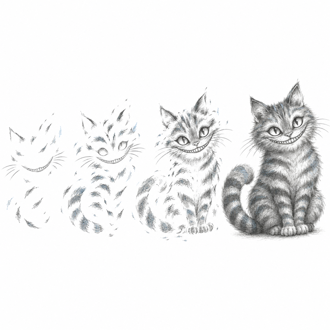
A cat becomes progressively more complete across four pencil sketches, suggesting a hierarchy of visual features.

Lecture map

  1. Images and local visual evidence
  2. Spatial control and feature hierarchies
  3. Deep convolutional architectures
  4. Using visual representations

Print / save as PDF

Part 1 · Images and local visual evidence

  1. Images and local visual evidence
  2. Spatial control and feature hierarchies
  3. Deep convolutional architectures
  4. Using visual representations

Why local connectivity and shared parameters fit many visual tasks.

From an MLP to a convolutional network

1

Prediction

𝒚̂=f(𝒙;θ)\widehat{\mathbf y}=f(\mathbf x;\theta)

→

2

Mean mini-batch objective

ℒℬ=1B∑i∈ℬℓi\mathcal L_{\mathcal B}=\frac{1}{B}\sum_{i\in\mathcal B}\ell_i

→

3

Gradient

∇θℒℬ\nabla_\theta\mathcal L_{\mathcal B}

→

4

Parameter update

θ←θ−η∇θℒℬ\theta\leftarrow\theta-\eta\nabla_\theta\mathcal L_{\mathcal B}

Week 04 · MLP

Every output unit can connect to every input value.

architecture changes →

Week 05 · CNN

Connections are local; the same parameters are shared across positions.

The learning loop stays the same; the architecture constrains which predictions it can express.

Images are structured measurements

One batch: 𝑿∈ℝB×Cin×H×W\mathbf X\in\mathbb R^{B\times C_{\mathrm{in}}\times H\times W}

CinC_{\mathrm{in}} measured channels H,WH,W spatial axes

Grayscale

Cin=1C_{\mathrm{in}}=1

One intensity at each location.

RGB

Cin=3C_{\mathrm{in}}=3

Three measurements at each location in one image.

Hyperspectral

Cin≫3C_{\mathrm{in}}\gg3

Many wavelength bands at each location.

Channels describe what is measured; height and width describe where it is measured.

Dense connectivity spends parameters on every location

Both layers map the same input to the same output shape:

1×28×28→8×28×281\times28\times28\ \longrightarrow\ 8\times28\times28

Dense layer

784 inputs≋≋≋≋≋6272 outputs

Each output has its own weight for every input.

784×6272+6272=𝟒,𝟗𝟐𝟑,𝟓𝟐𝟎784\times6272+6272=\mathbf{4{,}923{,}520}

Conv2d: 8 filters, 3×33\times3, padding 1

local 3×33\times3same filter
at every position
8 maps

Eight local filters are shared over the image.

8×1×3×3+8=𝟖𝟎8\times1\times3\times3+8=\mathbf{80}

Equal output dimensions do not mean equal models: the convolution imposes local, shared connectivity.

A historical experiment on visual selectivity
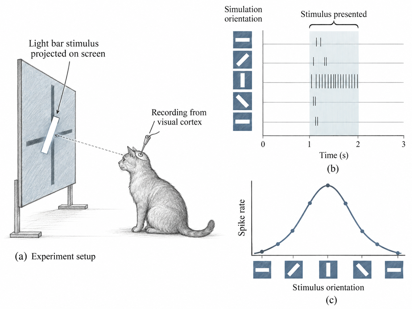
Unaltered instructor-supplied schematic of a cat viewing an oriented light bar while an electrode records from visual cortex; schematic spike trains and an orientation-tuning curve appear at right.

What was measured

Invasive single-cell recordings from visual cortex in lightly anaesthetized cats while patterned light stimulated the retina.

What this drawing shows

The spikes and tuning curve are schematic illustrations, not data reproduced from the paper.

Historical study: (Hubel and Wiesel 1959). Supplied schematic shown unaltered.

Biological evidence and the CNN design

Measured observation

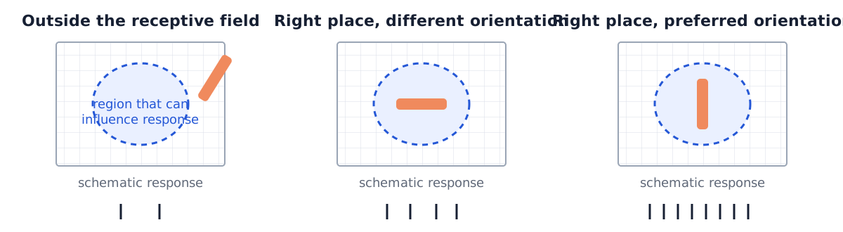
Some recorded cortical cells responded selectively to visual patterns in restricted regions.

motivates architectural questions →

⌗

Local connectivity

Each unit initially uses a small spatial neighborhood.

↔︎

Shared weights

One learned local rule is reused at many positions.

▱

Composition through layers

Deeper layers combine earlier local responses.

These are engineered CNN assumptions. The cat experiment did not prove them or prescribe a CNN.

Notation and vocabulary

Image batch

𝑿∈ℝB×Cin×H×W\mathbf X\in\mathbb R^{B\times C_{\mathrm{in}}\times H\times W}

Conv2d weights

𝑾∈ℝCout×Cin×kH×kW\mathbf W\in\mathbb R^{C_{\mathrm{out}}\times C_{\mathrm{in}}\times k_H\times k_W}

Preactivations

𝒛∈ℝB×Cout×Hout×Wout\mathbf z\in\mathbb R^{B\times C_{\mathrm{out}}\times H_{\mathrm{out}}\times W_{\mathrm{out}}}

Kernel slice

Spatial weights for one input channel.

Filter

All channel slices that produce one output channel.

Response map

Output of a fixed kernel before an activation.

Activation map

One channel of a learned representation after activation.

Single-layer notation suppresses (ℓ)(\ell): 𝒉=ϕ(𝒛)\mathbf h=\phi(\mathbf z), with 𝒉(0)=𝑿\mathbf h^{(0)}=\mathbf X.

Fixed kernels ask local questions

Local mean

19\frac1919\frac1919\frac19 19\frac1919\frac1919\frac19 19\frac1919\frac1919\frac19

Asks: what is the average intensity nearby?

Smooths small local changes.

Vertical contrast

−1-10011 −1-10011 −1-10011

Asks: does the right side exceed the left?

Produces a signed edge response.

A kernel defines one local question; scanning asks that same question at every position.

One kernel produces one grayscale response map
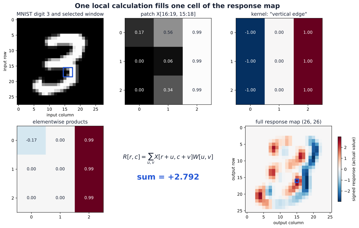
A genuine MNIST digit 3 has one three-by-three window outlined. Beside it are the selected patch, a vertical-edge kernel, elementwise products, their signed sum, and the complete response map with the matching output cell outlined.

One input channel

Cin=1C_{\mathrm{in}}=1

One fixed kernel

One signed scalar at each valid position.

Scan the image

Those scalars form one response map.

The map records where the kernel’s local pattern is present—and with which sign.

Learning chooses the local question
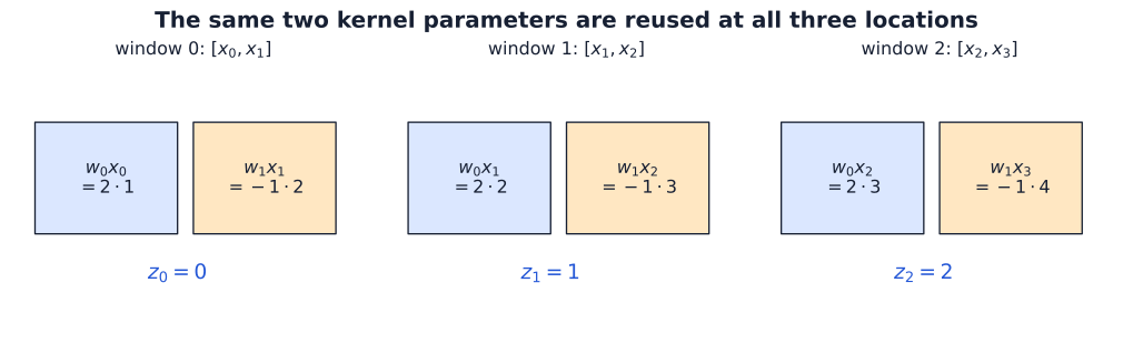
Three overlapping pairs from the input one, two, three, four use the same blue w-zero and orange w-one parameters, producing outputs zero, one, and two.

Forward pass

The same w0,w1w_0,w_1 participate at every position.

Backpropagation

Gradient contributions from all uses accumulate into ∇w0ℒ\nabla_{w_0}\mathcal L and ∇w1ℒ\nabla_{w_1}\mathcal L.

Update

One update changes the local question everywhere.

Weight sharing is a parameter identity built into the architecture; learning still uses the Week 04 loop.

Each RGB filter combines all input channels
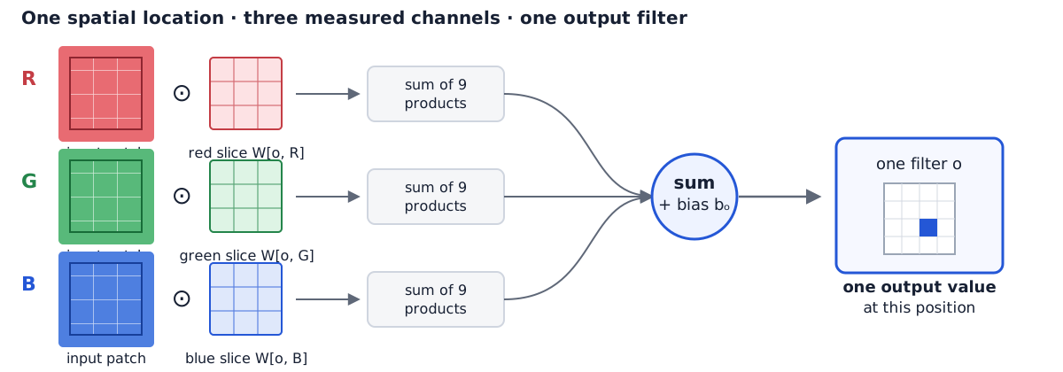
A flat diagram shows red, green, and blue input patches in parallel. Each is paired with its own kernel slice; the three channel contributions and one bias are summed into one output value for one filter.

One filter has shape Cin×kH×kWC_{\mathrm{in}}\times k_H\times k_W. For RGB, its three channel slices jointly produce one output value at each position.

RGB is one image with three measured channels; a filter combines them rather than classifying them independently.

Part 2 · Spatial control and feature hierarchies

  1. Images and local visual evidence
  2. Spatial control and feature hierarchies
  3. Deep convolutional architectures
  4. Using visual representations

How spatial sampling changes representations and how depth combines local evidence.

What does Conv2d compute?

input
B×Cin×H×WB\times C_{\mathrm{in}}\times H\times W
+ weights
Cout×Cin×kH×kWC_{\mathrm{out}}\times C_{\mathrm{in}}\times k_H\times k_W
→ preactivations
B×Cout×Hout×WoutB\times C_{\mathrm{out}}\times H_{\mathrm{out}}\times W_{\mathrm{out}}

groups=1, dilation=1; nn indexes examples, sH,sWs_H,s_W are strides.

zn,o,r,c=bo+∑i=0Cin−1∑u=0kH−1∑v=0kW−1Wo,i,u,vh̃n,i,rsH+u,csW+v. z_{n,o,r,c} =b_o+ \sum_{i=0}^{C_{\mathrm{in}}-1} \sum_{u=0}^{k_H-1} \sum_{v=0}^{k_W-1} W_{o,i,u,v}\, \widetilde h_{n,i,\,r s_H+u,\,c s_W+v}.

ii sums over all input channels.

u,vu,v sum over a local spatial window.

oo selects one learned output filter.

PyTorch uses unflipped cross-correlation; 𝒉̃\widetilde{\mathbf h} is the padded input, 𝒛\mathbf z the preactivation.

Operation convention: PyTorch Conv2d.

A structured linear map under the hood
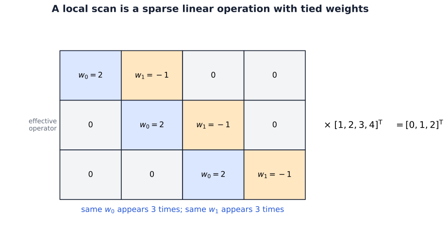
A three-by-four sparse matrix contains diagonally shifted copies of two shared parameters. It multiplies the four-value input to produce three responses.

Zeros encode locality

Each output ignores distant inputs.

Repeated labels encode sharing

The same parameter appears at shifted positions.

The operation is still linear

Before bias and activation, a convolution is a structured matrix multiplication.

Convolution restricts a dense linear map to a sparse, repeated pattern of coefficients.

Translation equivariance

Pattern at the left

filter →

translate input
four pixels →

The same pattern at the right

same filter →

f(TΔ𝒙)=TΔf(𝒙)f(T_{\Delta}\mathbf x)=T_{\Delta}f(\mathbf x)

For stride 1, shared weights make responses shift with the input, away from boundary effects.

Equivariance and classification invariance

Equivariant representation

shift input → feature map shifts

location is preserved

Invariant prediction

shift input → same class score

location is discarded

Convolution supplies a moving representation. Pooling, aggregation, data augmentation, and training determine whether the final decision becomes stable to a shift.

Equivariance is a property of the representation; invariance is a property of the final output.

Padding and boundary assumptions

A 33-value window centred at the left boundary needs one value outside the measured input.

No padding

outside47

Do not evaluate this boundary-centred window.

Zero padding

047

Assume the unmeasured value is zero.

Reflect padding

747

Assume the signal mirrors at the boundary.

Padding supplies values beyond the observed domain; its width controls output size and its rule changes border evidence.

Stride and spatial sampling

Stride s=1s=1

Evaluate every valid start: 0,1,2,3,4,5,60,1,2,3,4,5,6.

Stride s=2s=2

Evaluate starts 0,2,4,60,2,4,6; the others are skipped.

The filter is unchanged. The output samples fewer spatial positions, so a one-pixel input shift can land on a different sampling phase.

Stride reduces resolution by choosing where to evaluate the local rule.

Pooling and information loss

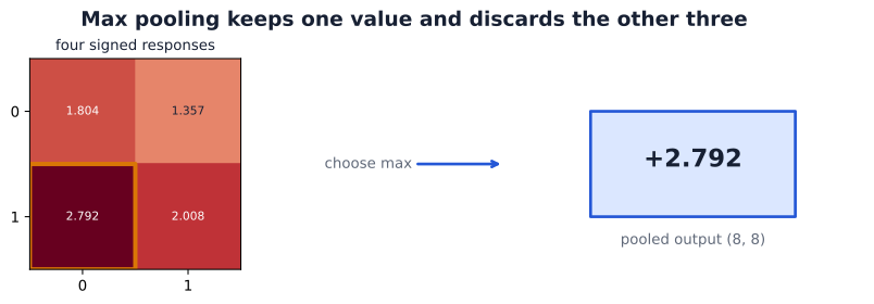
A two-by-two window contains four signed responses. The largest value, 2.792, is selected and written to one pooled output cell.

Max pooling keeps the largest value.

Average pooling keeps the local mean.

Both reduce a region to one number, discarding the exact arrangement inside that region.

Pooling can make some small shifts less consequential, but it does not guarantee translation invariance.

Pooling trades spatial detail for a compact summary.

Receptive fields through depth
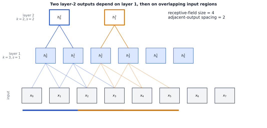
A three-level dependency graph shows input positions, width-three stride-one layer-one units, and two adjacent width-two stride-two layer-two units. Their paths end in overlapping four-position input regions whose starts are two positions apart.

Receptive-field size: four input positions can influence one layer-2 output.

Output spacing: adjacent layer-2 outputs begin two input positions apart.

Depth composes local dependencies into larger input regions; stride also changes how far adjacent outputs jump.

Receptive-field arithmetic

Track two quantities

One axis; sequential local layers; dilation 1.

jℓ=jℓ−1sℓ,rℓ=rℓ−1+(kℓ−1)jℓ−1. \begin{aligned} j_\ell &= j_{\ell-1}s_\ell,\\ r_\ell &= r_{\ell-1}+(k_\ell-1)j_{\ell-1}. \end{aligned}

rℓr_\ell: receptive-field size
jℓj_\ell: input spacing between adjacent outputs

Stage kk ss rr jj
input — — 1 1
layer 1 3 1 3 1
layer 2 2 2 4 2

For this two-layer path, one output sees four input positions while adjacent outputs are spaced two positions apart.

Feature hierarchies in a trained network
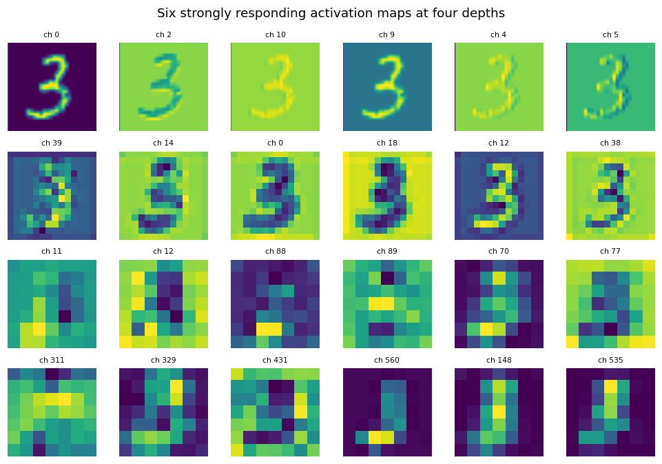
A four-by-six grid shows six strongly responding MobileNetV3-Small activation maps at four depths for one MNIST digit 3. Early maps preserve fine spatial detail; later maps are smaller and more abstract.

Early block

Fine spatial detail remains visible.

Deeper blocks

Resolution shrinks while channels combine earlier responses.

Interpret carefully

Strong activation does not give every channel a simple human-readable meaning.

Composition through layers changes both what a channel represents and how precisely it preserves location.

Spatial aggregation and class logits

C×H×WC\times H\times W
activation maps
→
1HW∑r,c\displaystyle \frac{1}{HW}\sum_{r,c}
one mean
per channel
→
[h‾1,…,h‾C][\bar h_1,\ldots,\bar h_C]
→
KK class logits

Retained: which channels responded strongly.

Discarded: where within each map the responses occurred.

Global average pooling creates location-insensitive summaries by explicitly removing spatial coordinates.

Convolution in one, two, and three dimensions

━━━━

Conv1d

Slides along one spatial axis: time, sequence position, or distance.

Input: (B,C,T)(B,C,T)

▦

Conv2d

Slides along height and width: images and spatial fields.

Input: (B,C,H,W)(B,C,H,W)

▧

Conv3d

Slides along three spatial axes: volumes or space–time grids.

Input: (B,C,D,H,W)(B,C,D,H,W)

The dimension counts convolved spatial axes; channels remain measurements or learned features at each location.

Evidence from the tutorial experiment
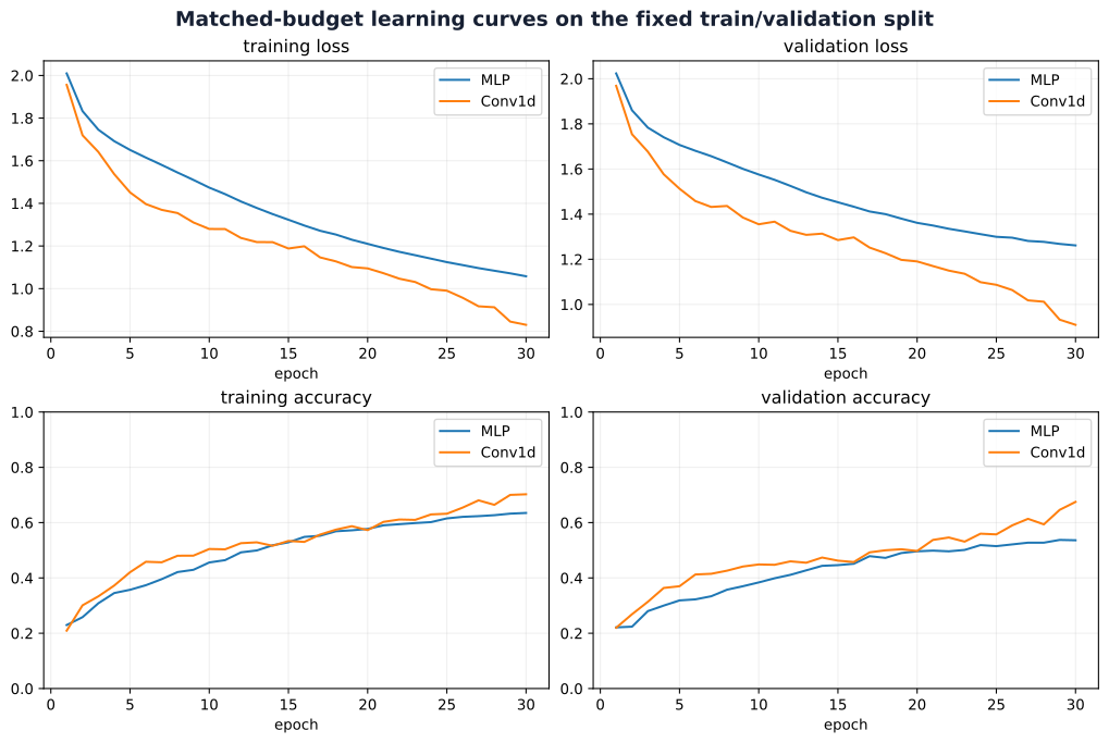
Four learning curves compare MLP and Conv1d training loss, validation loss, training accuracy, and validation accuracy over the same thirty epochs.

Accuracy · validation-selected epoch 30

Model Validation Test
MLP 0.536 0.521
Conv1d 0.675 0.654

Same split, seed, optimizer, and 30-epoch budget.

Both validation losses were still decreasing. This is one non-converged run on a synthetic benchmark—not a general ranking of CNNs and MLPs.

Here the local, shared architecture reached higher accuracy within 30 epochs; this does not establish faster wall-clock training.

When the convolutional bias fits

A useful match

  • nearby values interact meaningfully;
  • similar patterns recur across positions;
  • shifting a pattern should reuse the same rule;
  • larger structures can compose from local evidence.

A weak match

  • feature order is arbitrary;
  • absolute position changes the rule;
  • distant relationships dominate immediately;
  • the same pattern means different things by location.

Treat locality and sharing as hypotheses. Compare against credible alternatives with validation data and inspect failures under the shifts that matter.

CNNs work when their architectural assumptions resemble the structure of the task—not merely because the input can be arranged as a grid.

Part 3 · Deep convolutional architectures

  1. Images and local visual evidence
  2. Spatial control and feature hierarchies
  3. Deep convolutional architectures
  4. Using visual representations

Architectural choices that made deep visual models trainable.

AlexNet: a coordinated design

RGB crop→5 convolutional layers→3 fully connected layers→1000 classes

Use the available scale

1.2 million training images and two GPUs made a large model feasible.

Make optimization practical

ReLUs trained faster than saturating nonlinearities; pooling reduced spatial resolution.

Control overfitting

Random crops and reflections, colour augmentation, weight decay, and dropout.

ILSVRC 2012 top-5 test error: AlexNet ensemble 15.3% · second-best entry 26.2%

AlexNet’s result came from a coordinated model–data–compute–optimization system, not from convolution alone.

Architecture, training choices, and reported competition result: (Krizhevsky et al. 2012).

Reading the AlexNet paper

Follow the authors’ argument

Problem→design constraint→intervention→evidence

Open the original paper

Questions to carry into the paper

  1. Which choices increase representational capacity?
  2. Which choices make that capacity trainable on the available hardware?
  3. Which comparisons support each claimed benefit?

Architecture: five convolutional + three fully connected learned layers Optimization: ReLU comparison on CIFAR-10 Generalization: augmentation, dropout, held-out error

Read an architecture paper as a chain of design claims and evidence—not as a list of layers to memorize.

Guided reading: (Krizhevsky et al. 2012).

Original AlexNet and the Torchvision variant

2012 paper reportTraced Torchvision implementation

Input convention224×224×3224\times224\times3 stated; first response size needs an additional boundary convention1×3×224×2241\times3\times224\times224; padding 2 gives a reproducible 55×5555\times55 first response
Channels96 → 256 → 384 → 384 → 25664 → 192 → 384 → 256 → 256
Historical detailstwo-GPU grouped connectivity and local response normalizationsingle module graph; no local response normalization
Shared ideaconvolutional feature extractor followed by a large classifierthe same broad pattern, with implementation-specific dimensions

The name identifies a model family. It does not make a library implementation a literal reconstruction of the paper.

Paper specification: (Krizhevsky et al. 2012). Torchvision values come from the repository’s reviewed FX trace of alexnet(weights=None).

The optimization problem with increasing depth

If added layers can represent identity

trained shallow mapping+identity layers=same function

So its best achievable training error should be no worse.

But plain networks were harder to optimize

20-layer plain56-layer plain

On CIFAR-10, the deeper plain network showed higher training error.

Higher training error diagnoses an optimization problem; overfitting would instead describe a widening train–test gap.

When the shallow function can be preserved, extra depth need not worsen the best fit—but optimization may still struggle.

Constructed identity solution and 20/56-layer degradation experiment: (He et al. 2016). Bars are schematic, not digitized paper data.

Residual learning

𝒙\mathbf x
↗
↘
F(𝒙;θF)F(\mathbf x;\theta_F)learned correction𝒙\mathbf xidentity reference
+
𝒚\mathbf y

𝒚=F(𝒙;θF)+𝒙 \mathbf y=F(\mathbf x;\theta_F)+\mathbf x

If the desired mapping is near identity, learn a small correction. If identity is adequate, drive F(𝒙;θF)F(\mathbf x;\theta_F) toward zero.

The block learns what should change relative to its input, while the shortcut preserves a reference path.

Residual sum before a following activation; θF\theta_F collects branch parameters (He et al. 2016).

Information and gradients through a shortcut

Forward signal

𝒚=𝒙+F(𝒙)\mathbf y=\mathbf x+F(\mathbf x)

The block can preserve 𝒙\mathbf x directly while adding a learned transformation.

Backward sensitivity

∂𝒚∂𝒙=𝑰+∂F∂𝒙\dfrac{\partial\mathbf y}{\partial\mathbf x}=\mathbf I+\dfrac{\partial F}{\partial\mathbf x}

At the sum, the Jacobian has an identity term. A following ReLU adds its own gate.

This creates a useful route for signals and gradients. It does not guarantee convergence, prevent every vanishing gradient, or make arbitrary depth beneficial.

Addition lets the direct path and learned path coexist; optimization can use both.

Residual block definition: (He et al. 2016). The derivative follows from the block equation.

Identity and projection shortcuts

Identity shortcut: shapes already match
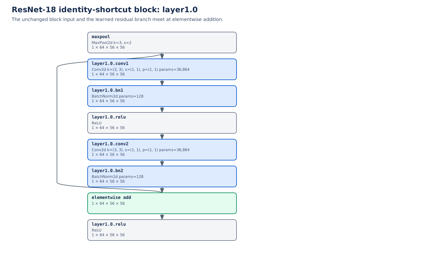
Automatically traced ResNet-18 layer one block zero: an unchanged identity shortcut and a two-convolution residual branch meet at elementwise addition.

shape⁡(𝒙)=shape⁡(F(𝒙))\operatorname{shape}(\mathbf x)=\operatorname{shape}(F(\mathbf x))

Projection shortcut: shape must change
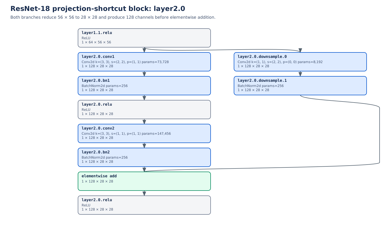
Automatically traced ResNet-18 layer two block zero: both the residual branch and a projection shortcut reduce spatial resolution and produce 128 channels before elementwise addition.

shape⁡(Ws𝒙)=shape⁡(F(𝒙))\operatorname{shape}(W_s\mathbf x)=\operatorname{shape}(F(\mathbf x))

Elementwise addition requires equal batch, channel, and spatial dimensions; a projection is used when they differ.

Automatically traced, untrained Torchvision ResNet-18 graphs; shortcut equations from (He et al. 2016).

The ResNet family
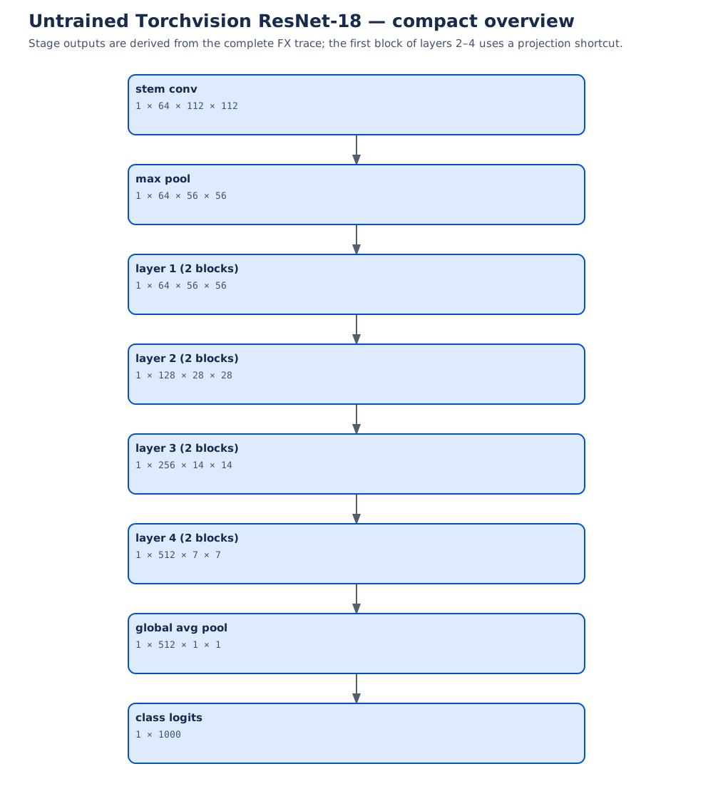
Compact automatically traced overview of untrained Torchvision ResNet-18, from its stem through four residual stages, global average pooling, and class logits.

Model Block Blocks per stage
ResNet-18 basic, 2 conv 2 · 2 · 2 · 2
ResNet-34 basic, 2 conv 3 · 4 · 6 · 3
ResNet-50 bottleneck, 3 conv 3 · 4 · 6 · 3
ResNet-101 bottleneck, 3 conv 3 · 4 · 23 · 3
ResNet-152 bottleneck, 3 conv 3 · 8 · 36 · 3

Across stages: spatial resolution falls while channel capacity rises.

The family scales depth by repeating residual blocks within a stable four-stage spatial design.

Family configurations and stage rules: (He et al. 2016). ResNet-18 overview is an automatically traced Torchvision implementation.

Why normalize activations?

1 · Centerx−μx-\mu→2 · Scale÷σ2+ϵ\div\sqrt{\sigma^2+\epsilon}→3 · Restore flexibilityγx̂+β\gamma\widehat{x}+\beta

μ,σ2\mu,\sigma^2 describe a chosen set of activations. ϵ>0\epsilon>0 prevents division by zero and limits extreme scaling. γ,β\gamma,\beta are learned with the rest of θ\theta.

Normalization changes the parameterization and optimization path. It does not guarantee unit variance after the learned affine step, nor does it make every deeper network train well.

The equation is shared; the method is defined by which activations contribute to μ\mu and σ2\sigma^2.

Batch-normalizing transform and learned affine parameters: (Ioffe and Szegedy 2015).

BatchNorm axes for image tensors

BBexamplesincluded
CCchannelskept separate
HHrowsincluded
WWcolumnsincluded

For each channel cc:

μc,σc2 use all xb,c,h,w over (b,h,w). \mu_c,\sigma_c^2\text{ use all }x_{b,c,h,w}\text{ over }(b,h,w).

One learned pair (γc,βc)(\gamma_c,\beta_c) is shared across spatial positions.

channel 0: its own statisticschannel 1: different statisticschannel 0 at another location: same statistics

BatchNorm2d(C) couples examples and locations within each channel; it does not mix channels into one mean.

Convolutional BatchNorm axes: (Ioffe and Szegedy 2015).

BatchNorm during training and evaluation

Training mode

current mini-batch→μℬ,σℬ2\mu_{\mathcal B},\sigma^2_{\mathcal B}→normalized output

The current batch affects every example’s output. Running estimates are updated for later evaluation.

Evaluation mode

one input→stored running statistics→deterministic output

The learned γ,β\gamma, \beta remain active, but the current evaluation batch does not set the statistics.

Small or correlated batches: noisy, unrepresentative training statistics. Domain shift: stored statistics may describe the pretraining domain poorly. Wrong mode: training and evaluation can silently disagree.

BatchNorm carries state: correct train/eval mode and representative batches are part of the model’s behavior.

Default track_running_stats=True: PyTorch BatchNorm2d; (Ioffe and Szegedy 2015).

LayerNorm for one example

Values𝒙=(1,3)\mathbf x=(1,3)
→
Statisticsμ=2\mu=2σ2=1\sigma^2=1
→
Normalizeϵ=0.25\epsilon=0.25𝒙̂=(−0.894,0.894)\widehat{\mathbf x}=(-0.894,0.894)
→
Learned affineγ=(2,0.5)\gamma=(2,0.5)β=(1,−1)\beta=(1,-1)𝒚=(−0.789,−0.553)\mathbf y=(-0.789,-0.553)

x̂j=xj−21+0.25,yj=γjx̂j+βj. \widehat{x}_j=\frac{x_j-2}{\sqrt{1+0.25}}, \qquad y_j=\gamma_j\widehat{x}_j+\beta_j.

ϵ=0.25\epsilon=0.25 is deliberately large so its numerical role is visible; production defaults are usually much smaller.

LayerNorm computes statistics from the chosen coordinates of this example, then learns how each normalized coordinate should be scaled and shifted.

LayerNorm construction: (Ba et al. 2016).

LayerNorm axes for visual tensors

normalized_shape names the trailing axes that share statistics. For tokens, NN is token count and DD is embedding width.

Image tensor (B,C,H,W)(B,C,H,W)LayerNorm((C,H,W))one μ,σ2\mu,\sigma^2 over every channel and pixel of each image
Per-channel spatial mapLayerNorm((H,W))separate μ,σ2\mu,\sigma^2 for each (b,c)(b,c) map
Vision-transformer tokens (B,N,D)(B,N,D)LayerNorm(D)separate μ,σ2\mu,\sigma^2 across features for each token

The affine parameter shape follows normalized_shape; changing the axes changes both the statistics and the learned degrees of freedom.

LayerNorm is batch-independent, but its meaning is incomplete until the normalized axes are stated.

Single-example LayerNorm principle: (Ba et al. 2016). Axis notation: PyTorch LayerNorm.

Choosing a normalization method

Choice Statistics over Batch coupling Train / eval Useful starting point
BatchNorm2d(C) B,H,WB,H,W for each cc yes different statistics CNN with representative batches
LayerNorm((C,H,W)) C,H,WC,H,W for each bb no same computation batch-independent whole-image features
LayerNorm(D) on (B,N,D)(B,N,D) DD for each (b,n)(b,n) no same computation token features (e.g. ViT)
no normalization none no same computation baseline to test on validation data

Choose axes that preserve distinctions the task needs, then test the choice under the actual batch size and deployment distribution.

Normalization is an architectural hypothesis about which activation scales may be treated as nuisance variation.

BatchNorm: (Ioffe and Szegedy 2015). LayerNorm: (Ba et al. 2016).

Part 4 · Using visual representations

  1. Images and local visual evidence
  2. Spatial control and feature hierarchies
  3. Deep convolutional architectures
  4. Using visual representations

Match invariances, pretraining, and model choice to the evidence available.

Augmentation expresses an invariance assumption

A plausible label-preserving change

CAT↔︎CAT

Horizontal reflection can preserve an object-class label.

A label-changing change

←↔︎→

Reflection reverses the meaning of a direction sign.

Training on T(𝒙)T(\mathbf x) with the original label asserts that y(T(𝒙))=y(𝒙)y(T(\mathbf x))=y(\mathbf x) for the task.

Use augmentation only when the transformation preserves the target and resembles variation expected after deployment.

AlexNet used random crops, reflections, and colour augmentation as task-specific regularization (Krizhevsky et al. 2012).

Frozen-feature transfer

Pretrained backbonesource-task features→𝒉\mathbf hfixed representation→New task headrandomly initialized→Target prediction

Frozen

Backbone parameters and normalization state stay fixed; use evaluation mode.

Trainable

Only the new head follows the gradient update.

Strong starting point when target labels or compute are limited and the source representation matches the target domain.

Frozen transfer tests whether an existing representation already separates the new task.

Feature transfer becomes less reliable as source and target tasks diverge (Yosinski et al. 2014).

Fine-tuning a pretrained representation

Strategy Updated parameters Adaptation Main risk
Head only new task head low representation mismatch
Partial head + later blocks medium unstable frozen/trainable boundary
Full entire network high overfitting or destructive updates

start with head only→unfreeze later blocks→fine-tune all layers if evidence supports it

Compare strategies on the same validation split. Use smaller learning rates for pretrained parameters and inspect domain-specific errors.

Fine-tuning trades preservation of reusable features for adaptation to the target task; validation chooses the useful amount.

Transferred initialization can improve generalization even after target-task fine-tuning (Yosinski et al. 2014).

CNNs, MLPs, and Vision Transformers

Starting assumption CNN Image MLP Vision Transformer
Input units pixels or features on a grid flattened pixels or patches embedded image patches
Early interaction local, shared filters dense or token-mixing layers self-attention can connect distant patches
Spatial prior strong locality and translation sharing depends on design position must be represented explicitly
Evidence to seek task matches local repeated patterns simple baseline is competitive pretraining, data, and compute justify weaker image-specific bias

These are typical starting assumptions, not permanent boundaries: hybrids and modern variants combine them.

Choose the architecture whose assumptions and resource needs match the task, then compare it against credible baselines.

ViT represents images as patch sequences and uses position embeddings; its original study found stronger dependence on pretraining scale than comparable CNNs (Dosovitskiy et al. 2021).

Evidence that a visual model works

1 · Held-out performancetask metric, calibration, and uncertainty
2 · Error structureper-class and subgroup failures
3 · Shortcut probesbackground, crop, colour, and occlusion tests
4 · Shifted conditionsnew devices, sites, seasons, or populations

Decision question: does the model keep using the right evidence when conditions change in ways that matter?

A high average score is the beginning of evaluation; deployment claims require failure analysis under realistic shifts.

Lecture synthesis

Local evidencesmall receptive fields→Shared filtersreuse across positions→Compositionlarger structures through depth→Aggregationtask-level prediction→Validationtest assumptions on data

Why CNN ideas work

They reduce the search space when locality, repetition, and hierarchy describe the task.

When they fail

The imposed invariances or connectivity can discard distinctions the target needs.

Architecture encodes a hypothesis about visual structure; training fits it, and held-out evidence decides whether it was useful.

Key dates and publications

1959 · Measured visual selectivity

Hubel and Wiesel characterize receptive fields in cat visual cortex.

1980 · Neocognitron

Fukushima proposes a hierarchical network designed for shift-tolerant pattern recognition.

1989 · Learned convolutional recognition

LeCun and colleagues train a constrained network for handwritten ZIP codes.

1998 · LeNet-5 and documents

Gradient-based convolutional systems are evaluated in practical document recognition.

2012–2016 · Scale and depth

AlexNet demonstrates GPU-scale ImageNet training; residual learning supports much deeper models.

2021 · Vision Transformer

Patch tokens and self-attention offer a scalable alternative visual architecture.

Progress came from changing architectural assumptions together with data, optimization, and compute.

Person of the day: Yann LeCun

Instructor-provided portrait of Yann LeCun.

Yann LeCun helped make trainable convolutional networks a practical approach to visual recognition.

1989 · Learn the filters

Task-specific architectural constraints and backpropagation support handwritten ZIP-code recognition (LeCun et al. 1989).

1998 · Build a recognition system

LeNet-5 connects learned convolutional features to document-reading applications (LeCun et al. 1998).

2018 · ACM A.M. Turing Award

LeCun shares the award with Geoffrey Hinton and Yoshua Bengio for conceptual and engineering breakthroughs in deep neural networks (Association for Computing Machinery, n.d.).

Local connectivity and shared parameters become useful when they are trained end to end for the task.

References

Association for Computing Machinery. n.d. “Yann LeCun: 2018 ACM A.M. Turing Award Laureate.” Accessed September 30, 2026. https://amturing.acm.org/award_winners/lecun_6017366.cfm.
Ba, Jimmy Lei, Jamie Ryan Kiros, and Geoffrey E. Hinton. 2016. “Layer Normalization.” arXiv Preprint arXiv:1607.06450. https://arxiv.org/abs/1607.06450.
Dosovitskiy, Alexey, Lucas Beyer, Alexander Kolesnikov, et al. 2021. “An Image Is Worth 16x16 Words: Transformers for Image Recognition at Scale.” International Conference on Learning Representations. https://arxiv.org/abs/2010.11929.
Fukushima, Kunihiko. 1980. “Neocognitron: A Self-Organizing Neural Network Model for a Mechanism of Pattern Recognition Unaffected by Shift in Position.” Biological Cybernetics 36: 193–202. https://doi.org/10.1007/BF00344251.
He, Kaiming, Xiangyu Zhang, Shaoqing Ren, and Jian Sun. 2016. “Deep Residual Learning for Image Recognition.” Proceedings of the IEEE Conference on Computer Vision and Pattern Recognition, 770–78. https://openaccess.thecvf.com/content_cvpr_2016/html/He_Deep_Residual_Learning_CVPR_2016_paper.html.
Hubel, David H., and Torsten N. Wiesel. 1959. “Receptive Fields of Single Neurones in the Cat’s Striate Cortex.” The Journal of Physiology 148 (3): 574–91. https://doi.org/10.1113/jphysiol.1959.sp006308.
Ioffe, Sergey, and Christian Szegedy. 2015. “Batch Normalization: Accelerating Deep Network Training by Reducing Internal Covariate Shift.” Proceedings of the 32nd International Conference on Machine Learning 37: 448–56. https://proceedings.mlr.press/v37/ioffe15.html.
Krizhevsky, Alex, Ilya Sutskever, and Geoffrey E. Hinton. 2012. “ImageNet Classification with Deep Convolutional Neural Networks.” Advances in Neural Information Processing Systems 25. https://papers.nips.cc/paper_files/paper/2012/hash/c399862d3b9d6b76c8436e924a68c45b-Abstract.html.
LeCun, Yann, Bernhard Boser, John S. Denker, et al. 1989. “Backpropagation Applied to Handwritten Zip Code Recognition.” Neural Computation 1 (4): 541–51. https://doi.org/10.1162/neco.1989.1.4.541.
LeCun, Yann, Léon Bottou, Yoshua Bengio, and Patrick Haffner. 1998. “Gradient-Based Learning Applied to Document Recognition.” Proceedings of the IEEE 86 (11): 2278–324. https://doi.org/10.1109/5.726791.
Yosinski, Jason, Jeff Clune, Yoshua Bengio, and Hod Lipson. 2014. “How Transferable Are Features in Deep Neural Networks?” Advances in Neural Information Processing Systems 27. https://papers.nips.cc/paper_files/paper/2014/hash/532a2f85b6977104bc93f8580abbb330-Abstract.html.

References — continued