Nonlinear representation learning
with feedforward neural networks

Week-04 ยท ML-2026

Alexei Kornaev,
Dr. Sc., Prof.

Innopolis University

Researcher at the RC for AI,
National RC for Oncology n.a. N.N. Blokhin

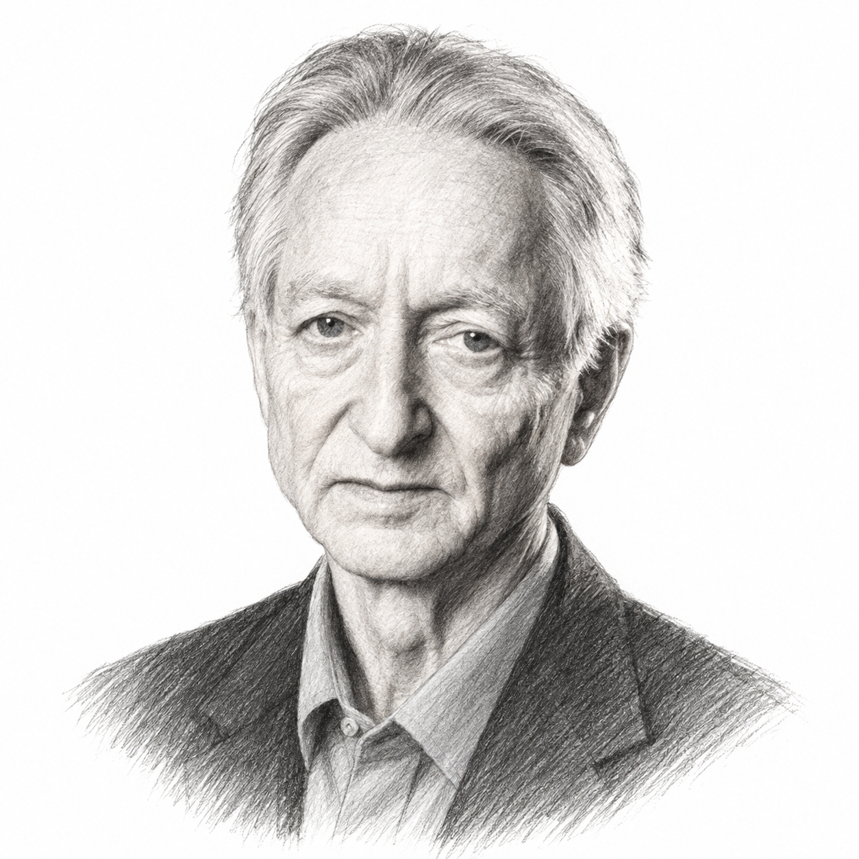
Instructor-supplied Week 04 graphical abstract for the neural-networks lecture.

Lecture map

  1. Learned representations and MLPs
  2. Forward propagation, outputs, and tasks
  3. Backpropagation and autograd
  4. Training and generalization

Print / save as PDF

Part 1 ยท Learned representations and MLPs

  1. Learned representations and MLPs
  2. Forward propagation, outputs, and tasks
  3. Backpropagation and autograd
  4. Training and generalization

From artificial neurons to nonlinear multilayer architectures.

Where are we in machine learning?

Model Prediction What is learned? Source of flexibility
Linear regression ๐’˜โŠค๐’™+b\mathbf w^\top\mathbf x+b Coefficients Linear response
Logistic regression ฯƒ(๐’˜โŠค๐’™+b)\sigma(\mathbf w^\top\mathbf x+b) Decision boundary Linear boundary in feature space
Decision tree Leaf value Splits and leaves Recursive partitioning
Forest / boosting Ensemble prediction Multiple trees Combined partitions
MLP f(L)โˆ˜โ‹ฏโˆ˜f(1)(๐’™)f^{(L)}\!\circ\cdots\circ f^{(1)}(\mathbf x) Transformations and predictor Learned nonlinear representation

The final row adds learned features between the supplied input and the prediction.

The learning algorithm remains the same

Logistic regression

yฬ‚=ฯƒ(๐’˜โŠค๐’™+b) \widehat y=\sigma(\mathbf w^\top\mathbf x+b)

Two-layer network

๐’‰=ฯ•(๐‘พ(1)๐’™+๐’ƒ(1)),yฬ‚=g(๐‘พ(2)๐’‰+๐’ƒ(2)) \mathbf h=\phi(\mathbf W^{(1)}\mathbf x+\mathbf b^{(1)}), \qquad \widehat y=g(\mathbf W^{(2)}\mathbf h+\mathbf b^{(2)})

ฮธโ†’yฬ‚โ†’โ„’โ†’โˆ‡ฮธโ„’โ†’ฮธโˆ’ฮทโˆ‡ฮธโ„’ \theta \longrightarrow \widehat y \longrightarrow \mathcal L \longrightarrow \nabla_\theta\mathcal L \longrightarrow \theta-\eta\nabla_\theta\mathcal L

ฮธ={๐‘พ(โ„“),๐’ƒ(โ„“)}โ„“=1L\theta=\{\mathbf W^{(\ell)},\mathbf b^{(\ell)}\}_{\ell=1}^{L} collects all trainable parameters. The output transformation gg depends on the prediction task.

The model becomes richer; the learning loop remains familiar.

The network learns the representation
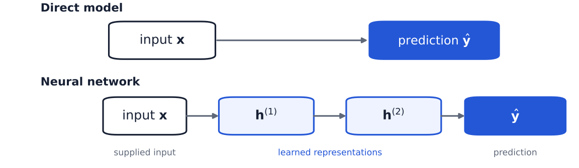
A supplied input passes directly to a prediction in one pipeline and through two learned hidden representations in another.

Earlier layers learn the features used by later layers.

Natural and artificial neurons
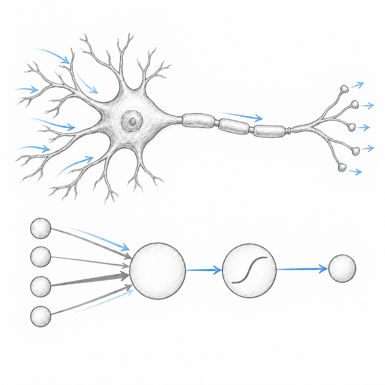
Instructor-provided comparison of a natural neuron and an artificial neuron.

Natural neuron. Receives electrochemical signals through dendrites and synapses, integrates them across space and time, and may generate an action potential transmitted along the axon.

Artificial neuron. Receives numerical inputs, scales them by learned weights, adds a bias, and applies an activation function to produce an output.

Biological terminology Artificial abstraction
Incoming signals Inputs xjx_j
Synaptic influence Weights wjw_j
Signal integration Weighted sum and bias
Firing response Activation function
Axon signal Output hh

This is a functional analogy, not a mechanistic model: biological neurons are dynamic, spiking, adaptive cells; an artificial neuron is a simplified differentiable computation.

An artificial neuron accumulates evidence
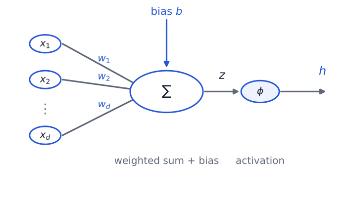
Inputs x one through x d enter a weighted sum with bias; activation phi transforms pre-activation z into output h.

z=๐’˜โŠค๐’™+b=โˆ‘j=1dwjxj+b,h=ฯ•(z). z=\mathbf w^\top\mathbf x+b = \sum_{j=1}^{d}w_jx_j+b, \qquad h=\phi(z).

The weighted sum collects signed evidence. The activation shapes the signal passed onward.

Activation functions shape the signal
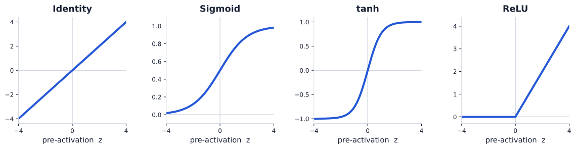
Four aligned plots show identity, sigmoid, tanh, and ReLU over pre-activation values from minus four to four.

ฯ•(z)=z\phi(z)=z
Range: โ„\mathbb R
Preserves the affine signal.

ฯ•(z)=11+eโˆ’z\phi(z)=\frac{1}{1+e^{-z}}
Range: (0,1)(0,1)
Maps scores to bounded positive outputs.

ฯ•(z)=tanhโกz\phi(z)=\tanh z
Range: (โˆ’1,1)(-1,1)
Produces a zero-centred bounded signal.

ฯ•(z)=maxโก(0,z)\phi(z)=\max(0,z)
Range: [0,โˆž)[0,\infty)
Keeps positive evidence and clips negative values.

Variants such as Leaky ReLU modify the inactive side while preserving a piecewise-linear form.

Without nonlinearity, depth disappears
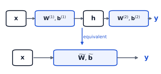
Two affine layers have the same input-output form as one equivalent affine layer.

๐’‰=๐‘พ(1)๐’™+๐’ƒ(1),๐’š=๐‘พ(2)๐’‰+๐’ƒ(2). \mathbf h=\mathbf W^{(1)}\mathbf x+\mathbf b^{(1)}, \qquad \mathbf y=\mathbf W^{(2)}\mathbf h+\mathbf b^{(2)}.

๐’š=๐‘พ(2)(๐‘พ(1)๐’™+๐’ƒ(1))+๐’ƒ(2)=(๐‘พ(2)๐‘พ(1))๐’™+(๐‘พ(2)๐’ƒ(1)+๐’ƒ(2)) \begin{aligned} \mathbf y &=\mathbf W^{(2)}(\mathbf W^{(1)}\mathbf x+\mathbf b^{(1)})+\mathbf b^{(2)}\\ &=(\mathbf W^{(2)}\mathbf W^{(1)})\mathbf x +(\mathbf W^{(2)}\mathbf b^{(1)}+\mathbf b^{(2)}) \end{aligned}

๐’š=๐‘พฬƒ๐’™+๐’ƒฬƒ. \mathbf y=\widetilde{\mathbf W}\mathbf x+\widetilde{\mathbf b}.

Two affine layers reduce to one equivalent affine layer.

Nonlinearity prevents a deep network from collapsing into a single affine transformation.

From one neuron to a layer
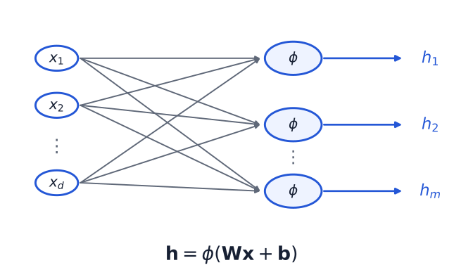
Several neurons receive the same input and produce activations collected into one vectorized layer.

Each neuron has its own weights and bias:

hi=ฯ•(๐’˜iโŠค๐’™+bi). h_i=\phi(\mathbf w_i^\top\mathbf x+b_i).

Stacking the neuron parameters gives one vectorized layer:

๐’‰=ฯ•(๐‘พ๐’™+๐’ƒ). \mathbf h=\phi(\mathbf W\mathbf x+\mathbf b).

The rows of ๐‘พ\mathbf W contain the neuronsโ€™ weight vectors.

Anatomy of a multilayer perceptron
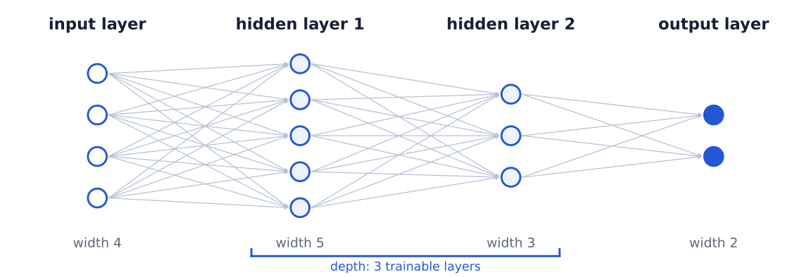
Feedforward network with four input units, hidden layers of widths five and three, and two output units.

4โ†’5โ†’3โ†’2,๐’‰(0)=๐’™,๐’‰(โ„“)=ฯ•(โ„“)(๐‘พ(โ„“)๐’‰(โ„“โˆ’1)+๐’ƒ(โ„“)). 4\longrightarrow5\longrightarrow3\longrightarrow2, \qquad \mathbf h^{(0)}=\mathbf x, \qquad \mathbf h^{(\ell)}= \phi^{(\ell)}\!\left(\mathbf W^{(\ell)}\mathbf h^{(\ell-1)}+\mathbf b^{(\ell)}\right).

Part 2 ยท Forward propagation, outputs, and tasks

  1. Learned representations and MLPs
  2. Forward propagation, outputs, and tasks
  3. Backpropagation and autograd
  4. Training and generalization

Follow values through the network and interpret its outputs.

Shapes are part of the mathematics

One sample

๐’›(โ„“)=๐‘พ(โ„“)๐’‰(โ„“โˆ’1)+๐’ƒ(โ„“). \mathbf z^{(\ell)}=\mathbf W^{(\ell)}\mathbf h^{(\ell-1)}+\mathbf b^{(\ell)}.

๐’‰(โ„“โˆ’1)โˆˆโ„dโ„“โˆ’1,๐‘พ(โ„“)โˆˆโ„dโ„“ร—dโ„“โˆ’1,๐’ƒ(โ„“),๐’›(โ„“)โˆˆโ„dโ„“. \begin{aligned} \mathbf h^{(\ell-1)}&\in\mathbb R^{d_{\ell-1}},\\ \mathbf W^{(\ell)}&\in\mathbb R^{d_\ell\times d_{\ell-1}},\\ \mathbf b^{(\ell)},\mathbf z^{(\ell)}&\in\mathbb R^{d_\ell}. \end{aligned}

Batch of BB samples

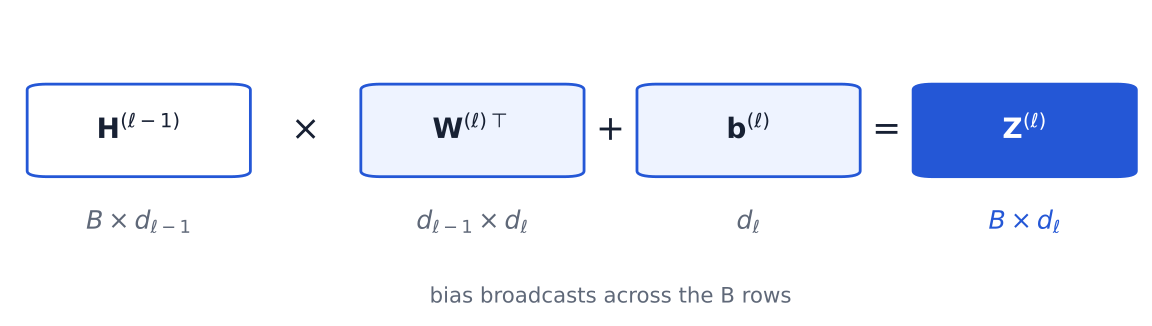
๐’(โ„“)=๐‘ฏ(โ„“โˆ’1)๐‘พ(โ„“)โŠค+๐’ƒ(โ„“)โˆˆโ„Bร—dโ„“. \mathbf Z^{(\ell)}=\mathbf H^{(\ell-1)}\mathbf W^{(\ell)\top}+\mathbf b^{(\ell)} \in\mathbb R^{B\times d_\ell}.

Batch-first matrix multiplication: B by input width times input width by output width, plus output-width bias, yields B by output width.

PyTorch stores each neuronโ€™s weights as one row of weight, with shape doutร—dind_{\text{out}}\times d_{\text{in}}.

One neuron: a numerical forward pass

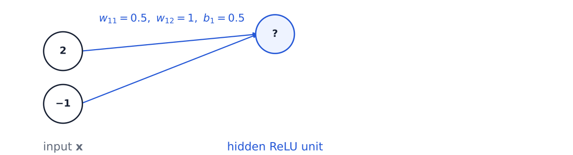
Two input values, 2 and minus 1, connect to one hidden ReLU neuron with its output initially left unknown.

๐’™=[2โˆ’1],๐’˜1=[0.51],b1=0.5. \mathbf x=\begin{bmatrix}2\\-1\end{bmatrix},\qquad \mathbf w_1=\begin{bmatrix}0.5\\1\end{bmatrix},\qquad b_1=0.5.

๐’˜1โŠค๐’™+b1=0.5(2)+1(โˆ’1)+0.5. \mathbf w_1^\top\mathbf x+b_1=0.5(2)+1(-1)+0.5.

z1=0.5.z_1=0.5.

h1=ReLUโก(0.5)=0.5.h_1=\operatorname{ReLU}(0.5)=0.5.

Calculate the weighted contributions before revealing the result.

One layer: neurons work in parallel
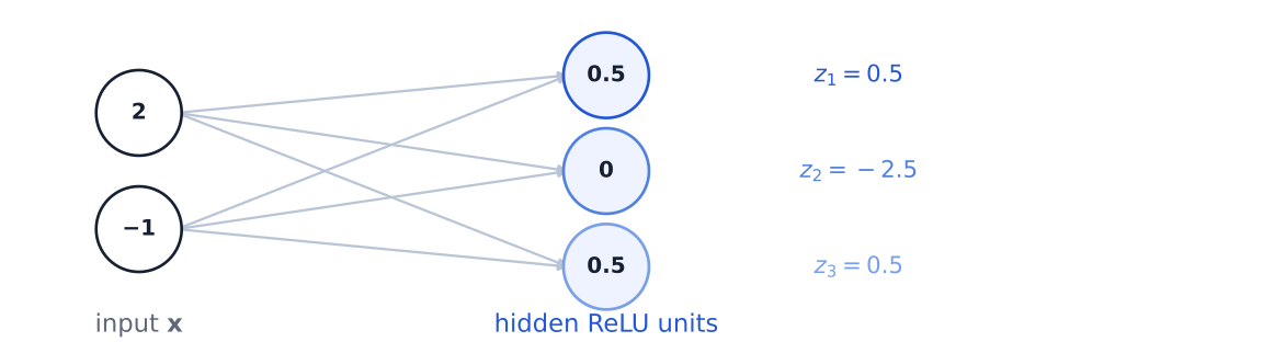
The same two inputs feed three ReLU neurons; their pre-activations are 0.5, minus 2.5, and 0.5, and outputs are 0.5, 0, and 0.5.

๐‘พ(1)=[0.51โˆ’10.511],๐’ƒ(1)=[0.50โˆ’0.5]. \mathbf W^{(1)}= \begin{bmatrix} 0.5&1\\-1&0.5\\1&1 \end{bmatrix},\qquad \mathbf b^{(1)}=\begin{bmatrix}0.5\\0\\-0.5\end{bmatrix}.

๐’›(1)=๐‘พ(1)๐’™+๐’ƒ(1)=[0.5โˆ’2.50.5]. \mathbf z^{(1)}=\mathbf W^{(1)}\mathbf x+\mathbf b^{(1)} =\begin{bmatrix}0.5\\-2.5\\0.5\end{bmatrix}.

๐’‰(1)=ReLUโก(๐’›(1))=[0.500.5]. \mathbf h^{(1)}=\operatorname{ReLU}(\mathbf z^{(1)}) =\begin{bmatrix}0.5\\0\\0.5\end{bmatrix}.

A layer performs several neuron calculations in one matrix operation.

A complete MLP forward pass
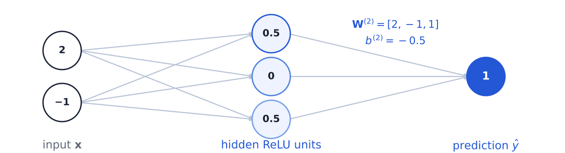
Complete two-to-three-to-one network: input 2 and minus 1, hidden values 0.5, 0, 0.5, and final prediction 1.

๐‘พ(2)=[2โˆ’11],b(2)=โˆ’0.5. \mathbf W^{(2)}=\begin{bmatrix}2&-1&1\end{bmatrix}, \qquad b^{(2)}=-0.5.

yฬ‚=๐‘พ(2)๐’‰(1)+b(2)=2(0.5)โˆ’1(0)+1(0.5)โˆ’0.5=1. \begin{aligned} \hat y &=\mathbf W^{(2)}\mathbf h^{(1)}+b^{(2)}\\ &=2(0.5)-1(0)+1(0.5)-0.5\\ &=1. \end{aligned}

Blue labels mark stored parameters; circles show intermediate values and the final prediction.

Forward propagation composes affine transformations with hidden-layer activations; the output transformation depends on the task.

From network outputs to predictions

Task Network output Interpretation Typical loss
Regression KK real values Predicted quantities MSE
Binary classification One logit zz p(y=1โˆฃx)=ฯƒ(z)p(y=1\mid x)=\sigma(z) BCE with logits
Multiclass classification KK logits Softmax probabilities; class argโกmaxโกkzk\arg\max_k z_k Cross-entropy

BCEWithLogitsLoss and CrossEntropyLoss expect logits and apply the required stable transformation internally.

argโกmaxโกksoftmaxโก(๐’›)k=argโกmaxโกkzk\arg\max_k\operatorname{softmax}(\mathbf z)_k=\arg\max_k z_k.

What does nn.Linear compute?

๐’=๐‘ฟ๐‘พโŠค+๐’ƒ.\mathbf Z=\mathbf X\mathbf W^\top+\mathbf b.

X                  (B, 2)
layer.weight       (3, 2)
layer.bias         (3,)
Z                  (B, 3)
layer = nn.Linear(
    in_features=2, out_features=3
)

Z = layer(X)
Z_explicit = (
    X @ layer.weight.T + layer.bias
)

torch.testing.assert_close(Z, Z_explicit)

nn.Linear performs the affine transformation. The activation is a separate operation.

Softmax turns logits into probabilities
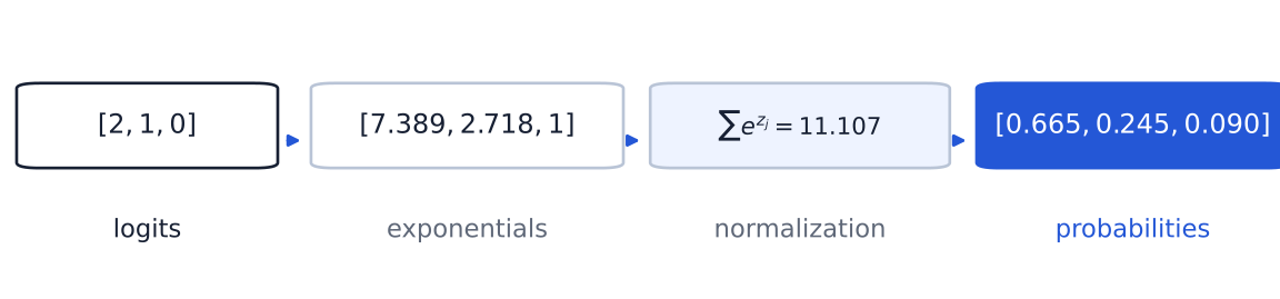
Navy logits 2, 1, 0 become exponentials and then blue class probabilities 0.665, 0.245, 0.090 after normalization.

๐’›i=[zi1,โ€ฆ,ziK]โˆˆโ„K,qik=qฮธ(y=kโˆฃ๐’™i)=expโก(zik)โˆ‘j=1Kexpโก(zij). \mathbf z_i=[z_{i1},\ldots,z_{iK}]\in\mathbb R^K, \qquad q_{ik}=q_\theta(y=k\mid\mathbf x_i) =\frac{\exp(z_{ik})}{\sum_{j=1}^{K}\exp(z_{ij})}.

qik>0,โˆ‘k=1Kqik=1,softmaxโก(๐’›+c๐Ÿ)=softmaxโก(๐’›).q_{ik}>0,\qquad\sum_{k=1}^{K}q_{ik}=1,\qquad \operatorname{softmax}(\mathbf z+c\mathbf 1)=\operatorname{softmax}(\mathbf z).

Softmax converts relative evidence into a categorical probability distribution.

Numerically stable implementations subtract the largest logit before exponentiation.

Softmax and cross-entropy complete the classifier

Model output

qik=softmaxโก(๐’›i)k.q_{ik}=\operatorname{softmax}(\mathbf z_i)_k.

๐’›=[2,1,0]โ†’๐’’โ‰ˆ[0.665,0.245,0.090].\mathbf z=[2,1,0]\quad\longrightarrow\quad\mathbf q\approx[0.665,0.245,0.090].

Observed class

๐’ši=[yi1,โ€ฆ,yiK],yikโˆˆ{0,1},โˆ‘k=1Kyik=1.\mathbf y_i=[y_{i1},\ldots,y_{iK}],\quad y_{ik}\in\{0,1\},\quad\sum_{k=1}^{K}y_{ik}=1.

๐’š=[0,1,0].\mathbf y=[0,1,0].

โ„“i=โˆ’โˆ‘k=1Kyiklogโกqik=โˆ’logโกqi,ci,โ„“=โˆ’logโก(0.245)โ‰ˆ1.41.\ell_i=-\sum_{k=1}^{K}y_{ik}\log q_{ik}=-\log q_{i,c_i}, \qquad\ell=-\log(0.245)\approx1.41.

The one-hot target selects the log-probability assigned to the observed class. Higher probability gives a smaller loss; lower probability gives a larger loss.

loss = F.cross_entropy(logits, targets)

logits (B,K)(B,K) ยท targets (B,)(B,) integer class indices

cross_entropy expects logits. It applies a stable log-softmax and negative log-likelihood internally (PyTorch contributors, n.d.-b).

How to read an architecture

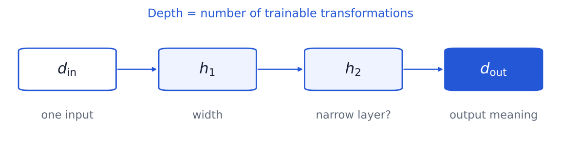
Generic input, two hidden widths, and output architecture annotated with input meaning, width, depth, and output interpretation.

  1. What does one input represent?
  2. What does the output dimension represent?
  3. Where are the wide and narrow layers?
  4. Is there a bottleneck or symmetry?
  5. Which output transformation and loss complete the model?

An architecture describes a mapping; the data, output interpretation, and loss define the task.

Guess the task: function approximator
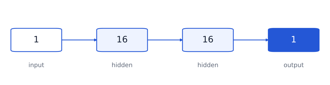
Architecture with widths 1, 16, 16, and 1; the task is initially withheld for students to guess.

Scalar input xx and target y=f(x)y=f(x) suggest regression or function approximation.

Linear output; typical loss: MSE.

Guess the task: image classifier
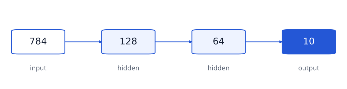
Architecture with widths 784, 128, 64, and 10; the task is initially withheld for students to guess.

784=28ร—28784=28\times28 grayscale pixels enter two learned hidden representations. Ten output logits suggest multiclass classification; typical loss: cross-entropy.

The dimensions suggest an MNIST-like task, but architecture alone does not identify the dataset.

Guess the task: autoencoder
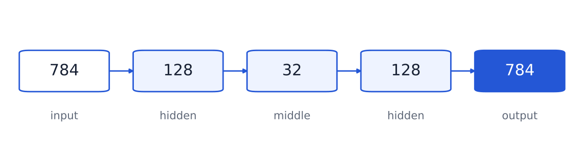
Approximately symmetric architecture with widths 784, 128, 32, 128, and 784, with a 32-dimensional bottleneck.

๐’™โ†’encoder๐’›โ†’decoder๐’™ฬ‚. \mathbf x\xrightarrow{\text{encoder}}\mathbf z \xrightarrow{\text{decoder}}\hat{\mathbf x}.

Matching input and output dimensions, approximate symmetry, and a 3232-dimensional bottleneck suggest reconstruction. The learned representation can also support dimensionality reduction or anomaly detection.

The bottleneck asks the network to preserve useful information in a smaller representation.

Part 3 ยท Backpropagation and autograd

  1. Learned representations and MLPs
  2. Forward propagation, outputs, and tasks
  3. Backpropagation and autograd
  4. Training and generalization

Use the chain rule to assign sensitivity to every parameter.

Learning asks who caused the error

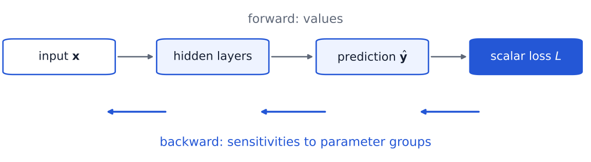
Data and predictions move forward to one scalar loss; sensitivity signals travel backward toward parameter groups.

๐’šฬ‚=fฮธ(๐’™),L=โ„’(๐’šฬ‚,๐’š), \hat{\mathbf y}=f_\theta(\mathbf x),\qquad L=\mathcal L(\hat{\mathbf y},\mathbf y),

โˆ‡ฮธL=[โˆ‚Lโˆ‚ฮธ1,โ€ฆ,โˆ‚Lโˆ‚ฮธP]. \nabla_\theta L=\left[ \frac{\partial L}{\partial\theta_1},\ldots, \frac{\partial L}{\partial\theta_P} \right].

How much would the loss change if this parameter changed slightly?

A computation graph remembers the forward pass
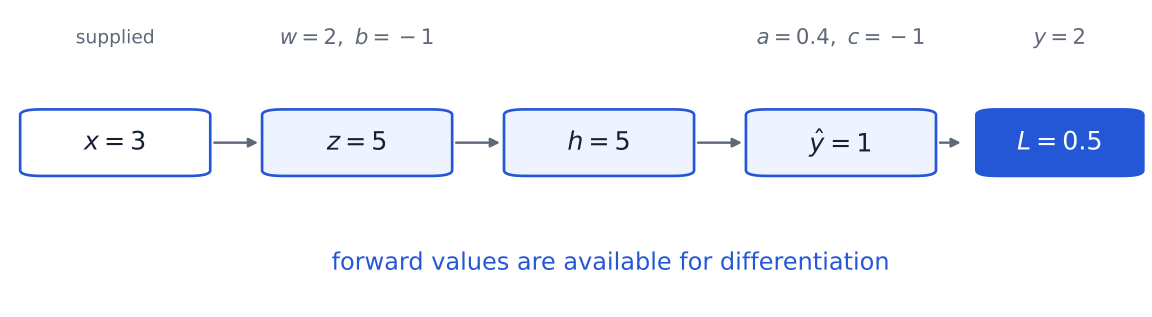
Fixed computation graph with supplied x equals 3 and y equals 2, trainable w equals 2, b equals minus 1, a equals 0.4, c equals minus 1, and forward values z equals 5, h equals 5, prediction equals 1, loss equals 0.5.

z=wx+b=5โ†’h=ReLUโก(z)=5โ†’yฬ‚=ah+c=1โ†’L=12(yฬ‚โˆ’y)2=0.5. z=wx+b=5\;\longrightarrow\; h=\operatorname{ReLU}(z)=5\;\longrightarrow\; \hat y=ah+c=1\;\longrightarrow\; L=\tfrac12(\hat y-y)^2=0.5.

Supplied: x=3,y=2x=3,y=2. Trainable: w=2,b=โˆ’1,a=0.4,c=โˆ’1w=2,b=-1,a=0.4,c=-1.

The backward pass uses the graph structure and selected values produced during the forward pass.

Every operation contributes a local derivative
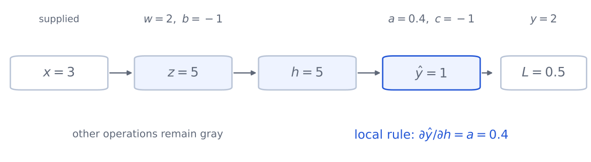
The same scalar graph is gray except the output operation, which is highlighted in blue for its local derivative.

โˆ‚Lโˆ‚yฬ‚=yฬ‚โˆ’y=โˆ’1,โˆ‚yฬ‚โˆ‚h=a=0.4. \frac{\partial L}{\partial\hat y}=\hat y-y=-1, \qquad \frac{\partial\hat y}{\partial h}=a=0.4. โˆ‚yฬ‚โˆ‚a=h=5,โˆ‚yฬ‚โˆ‚c=1. \frac{\partial\hat y}{\partial a}=h=5, \qquad \frac{\partial\hat y}{\partial c}=1.

โˆ‚hโˆ‚z=1(z=5>0), \frac{\partial h}{\partial z}=1\quad(z=5>0), โˆ‚zโˆ‚w=x=3,โˆ‚zโˆ‚b=1. \frac{\partial z}{\partial w}=x=3, \qquad \frac{\partial z}{\partial b}=1.

Each operation combines its local derivative with the sensitivity arriving from later operations.

The chain rule follows a path
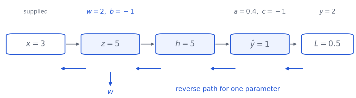
The scalar graph highlights a reverse dependency path from loss through prediction, h, z, and finally weight w.

โˆ‚Lโˆ‚w=โˆ‚Lโˆ‚yฬ‚โˆ‚yฬ‚โˆ‚hโˆ‚hโˆ‚zโˆ‚zโˆ‚w=(โˆ’1)(0.4)(1)(3)=โˆ’1.2. \frac{\partial L}{\partial w} =\frac{\partial L}{\partial\hat y} \frac{\partial\hat y}{\partial h} \frac{\partial h}{\partial z} \frac{\partial z}{\partial w} =(-1)(0.4)(1)(3)=-1.2.

Along a dependency path, local derivatives multiply.

Branches accumulate responsibility
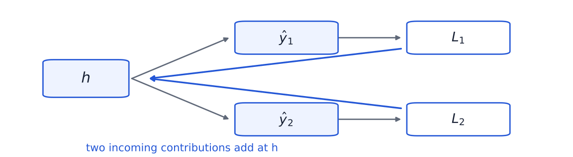
One hidden representation h feeds two prediction heads and two losses; blue paths return and meet at h.

hโ†’yฬ‚1โ†’L1,hโ†’yฬ‚2โ†’L2,L=L1+L2. h\longrightarrow\hat y_1\longrightarrow L_1, \qquad h\longrightarrow\hat y_2\longrightarrow L_2, \qquad L=L_1+L_2. โˆ‚Lโˆ‚h=โˆ‚L1โˆ‚h+โˆ‚L2โˆ‚h. \frac{\partial L}{\partial h} =\frac{\partial L_1}{\partial h} +\frac{\partial L_2}{\partial h}.

Along paths, derivatives multiply; where paths meet, gradient contributions add.

One complete forward and backward pass
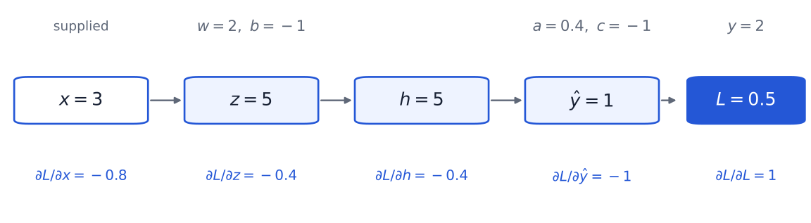
The original scalar graph displays forward values in navy and backward sensitivities in blue, including input sensitivity minus 0.8.

Forward values

Quantity Value
zz 55
hh 55
yฬ‚\hat y 11
LL 0.50.5

Backward sensitivities

Gradient Value Gradient Value
โˆ‚L/โˆ‚yฬ‚\partial L/\partial\hat y โˆ’1-1 โˆ‚L/โˆ‚a\partial L/\partial a โˆ’5-5
โˆ‚L/โˆ‚h\partial L/\partial h โˆ’0.4-0.4 โˆ‚L/โˆ‚c\partial L/\partial c โˆ’1-1
โˆ‚L/โˆ‚z\partial L/\partial z โˆ’0.4-0.4 โˆ‚L/โˆ‚w\partial L/\partial w โˆ’1.2-1.2
โˆ‚L/โˆ‚x\partial L/\partial x โˆ’0.8-0.8 โˆ‚L/โˆ‚b\partial L/\partial b โˆ’0.4-0.4

Forward propagation computes values. Backpropagation computes sensitivities.

Backpropagation through one layer
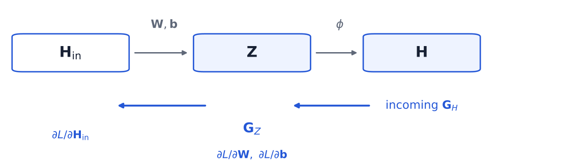
๐’=๐‘ฏin๐‘พโŠค+๐’ƒ,๐‘ฏ=ฯ•(๐’),๐‘ฎH=โˆ‚Lโˆ‚๐‘ฏ. \mathbf Z=\mathbf H_{\mathrm{in}}\mathbf W^\top+\mathbf b, \qquad \mathbf H=\phi(\mathbf Z), \qquad \mathbf G_H=\frac{\partial L}{\partial\mathbf H}.

๐‘ฎZ=๐‘ฎHโŠ™ฯ•โ€ฒ(๐’),โˆ‚Lโˆ‚๐‘พ=๐‘ฎZโŠค๐‘ฏin,โˆ‚Lโˆ‚๐’ƒ=โˆ‘i=1B๐‘ฎZ,i,โˆ‚Lโˆ‚๐‘ฏin=๐‘ฎZ๐‘พ. \begin{aligned} \mathbf G_Z&=\mathbf G_H\odot\phi'(\mathbf Z),\\ \frac{\partial L}{\partial\mathbf W}&=\mathbf G_Z^\top\mathbf H_{\mathrm{in}},\\ \frac{\partial L}{\partial\mathbf b}&=\sum_{i=1}^{B}\mathbf G_{Z,i},\\ \frac{\partial L}{\partial\mathbf H_{\mathrm{in}}}&=\mathbf G_Z\mathbf W. \end{aligned}

One matrix layer receives a sensitivity at its output, computes parameter gradients, and sends a sensitivity to its input.

Quantity Shape
๐‘ฏin\mathbf H_{\mathrm{in}} Bร—dinB\times d_{\mathrm{in}}
๐‘พ\mathbf W doutร—dind_{\mathrm{out}}\times d_{\mathrm{in}}
๐‘ฎZ\mathbf G_Z Bร—doutB\times d_{\mathrm{out}}
โˆ‚L/โˆ‚๐‘พ\partial L/\partial\mathbf W doutร—dind_{\mathrm{out}}\times d_{\mathrm{in}}
โˆ‚L/โˆ‚๐‘ฏin\partial L/\partial\mathbf H_{\mathrm{in}} Bร—dinB\times d_{\mathrm{in}}

Incoming sensitivity ๐‘ฎH\mathbf G_H โ†’ parameter gradients โ†’ sensitivity to the previous layer.

Backpropagation through an MLP
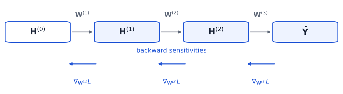
Activations move left to right through three trainable layers; sensitivities and parameter gradients move right to left.

๐‘ฎZ(โ„“)=๐‘ฎH(โ„“)โŠ™ฯ•โ€ฒ(๐’(โ„“)),โˆ‡๐‘พ(โ„“)L=๐‘ฎZ(โ„“)โŠค๐‘ฏ(โ„“โˆ’1),๐‘ฎH(โ„“โˆ’1)=๐‘ฎZ(โ„“)๐‘พ(โ„“). \begin{aligned} \mathbf G_Z^{(\ell)} &=\mathbf G_H^{(\ell)}\odot\phi'(\mathbf Z^{(\ell)}),\\ \nabla_{\mathbf W^{(\ell)}}L &=\mathbf G_Z^{(\ell)\top}\mathbf H^{(\ell-1)},\\ \mathbf G_H^{(\ell-1)} &=\mathbf G_Z^{(\ell)}\mathbf W^{(\ell)}. \end{aligned}

Backpropagation repeats the same layer-level calculation in reverse order.

Reverse-mode differentiation computes vectorโ€“Jacobian products without constructing every full Jacobian explicitly.

Autograd executes the graph backward

x = torch.tensor(3.0)
y = torch.tensor(2.0)

w = torch.tensor(2.0, requires_grad=True)
b = torch.tensor(-1.0, requires_grad=True)
a = torch.tensor(0.4, requires_grad=True)
c = torch.tensor(-1.0, requires_grad=True)

z = w * x + b
h = torch.relu(z)
y_hat = a * h + c
loss = 0.5 * (y_hat - y) ** 2

loss.backward()

โˆ‚Lโˆ‚L=1 \frac{\partial L}{\partial L}=1

The scalar loss seeds the backward pass.

w.grad = -1.2
b.grad = -0.4
a.grad = -5.0
c.grad = -1.0

PyTorch accumulates .grad on leaf tensors with requires_grad=True. Intermediate gradients can be retained explicitly (PyTorch contributors, n.d.-a).

What does x.grad compute?

x.grad=โˆ‚Lโˆ‚x=โˆ‚Lโˆ‚zโˆ‚zโˆ‚x=(โˆ’0.4)(2)=โˆ’0.8. x.\mathrm{grad}=\frac{\partial L}{\partial x} =\frac{\partial L}{\partial z} \frac{\partial z}{\partial x} =(-0.4)(2)=-0.8.

x = torch.tensor(3.0, requires_grad=True)
# same forward pass as before
loss.backward()
x.grad  # tensor(-0.8000)
Tensor Interpretation
w.grad Loss sensitivity to a trainable weight; used by the optimizer
x.grad Loss sensitivity to the input
z.grad Not stored by default: zz is a non-leaf intermediate
loss Seeds backward with โˆ‚L/โˆ‚L=1\partial L/\partial L=1

Call z.retain_grad() before backward() to store an intermediate gradient. Input gradients support sensitivity analysis, saliency, adversarial methods, and input optimization (PyTorch contributors, n.d.-a).

Checking and interpreting gradients

Central finite difference

โˆ‚Lโˆ‚ฮธiโ‰ˆL(ฮธi+ฮต)โˆ’L(ฮธiโˆ’ฮต)2ฮต. \frac{\partial L}{\partial\theta_i} \approx \frac{L(\theta_i+\varepsilon)-L(\theta_i-\varepsilon)}{2\varepsilon}.

For the running example:

โˆ‚Lโˆ‚wโ‰ˆโˆ’1.2.\frac{\partial L}{\partial w}\approx-1.2.

Observation Possible interpretation
Gradient near zero Saturation, inactive path, convergence, or weak sensitivity
Very large gradient Exploding gradient or poor scaling
No gradient stored Backward has not run, gradients are disabled, the tensor is disconnected, or a non-leaf gradient was not retained
NaN or Inf Numerical instability

A gradient measures local sensitivity and provides a diagnostic signal; its negative gives the steepest-descent direction.

Part 4 ยท Training and generalization

  1. Learned representations and MLPs
  2. Forward propagation, outputs, and tasks
  3. Backpropagation and autograd
  4. Training and generalization

Turn gradients into useful learning and evaluate what generalizes.

From gradients to a training loop

๐’€ฬ‚=fฮธ(๐‘ฟB),LB=1Bโˆ‘iโˆˆBโ„’(๐’šฬ‚i,๐’ši),ฮธt+1=ฮธtโˆ’ฮทโˆ‡ฮธLฬ‚Bt. \hat{\mathbf Y}=f_\theta(\mathbf X_B),\qquad L_B=\frac{1}{B}\sum_{i\in B}\mathcal L(\hat{\mathbf y}_i,\mathbf y_i),\qquad \theta_{t+1}=\theta_t-\eta\,\widehat{\nabla_\theta L}_{B_t}.

  1. Sample a mini-batch.
  2. Compute predictions.
  3. Compute the loss.
  4. Clear old gradients.
  5. Backpropagate.
  6. Update parameters.
  7. Repeat.
for X, y in loader:
    optimizer.zero_grad()

    y_hat = model(X)
    loss = criterion(y_hat, y)

    loss.backward()
    optimizer.step()

Autograd computes gradients; the optimizer uses them to change the parameters.

PyTorch accumulates gradients, so clear them before the next backward pass (PyTorch contributors, n.d.-d, n.d.-e).

The loss surface is not the training trajectory

Contours of one two-dimensional objective with a blue descent trajectory and local negative-gradient direction.

โˆ‡ฮธL(ฮธt)local information\nabla_\theta L(\theta_t)\quad\text{local information} ฮธ0,ฮธ1,โ€ฆ,ฮธTresulting trajectory\theta_0,\theta_1,\ldots,\theta_T\quad\text{resulting trajectory}

The objective defines the landscape; the training procedure determines how we move through it.

The surface depends on the model, data, and objective. The trajectory also depends on initialization, mini-batches, learning rate, and optimizer state. A two-dimensional contour is only a slice or projection.

The learning rate controls every step
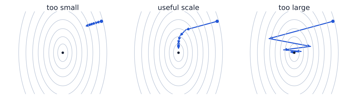
The same contours and starting point in three panels: small, useful-scale, and overly large learning rates.

gt=โˆ‡ฮธLฬ‚Bt,ฮ”ฮธt=โˆ’ฮทgt.g_t=\widehat{\nabla_\theta L}_{B_t},\qquad \Delta\theta_t=-\eta g_t.

The gradient measures local sensitivity; its negative supplies the descent direction, and the learning rate controls the update scale.

Too small can be slow; too large can overshoot or diverge. There is no universally optimal learning rate.

What does an optimizer change?
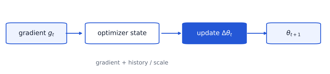
A mini-batch gradient enters an optimizer with state, which produces a parameter update.

Optimizer Main mechanism Practical consequence
SGD Current mini-batch gradient Simple; sensitive to learning rate and scale
Momentum Accumulates a moving direction Reduces oscillation and preserves motion
Adam Adaptive first- and second-moment estimates Often convenient and fast early in training
AdamW Adam with decoupled weight decay Shrinkage is separate from adaptive gradient scaling

gt=โˆ‡ฮธLฬ‚Bt,vt=ฮฒvtโˆ’1+gt,ฮธt+1=ฮธtโˆ’ฮทvt.g_t=\widehat{\nabla_\theta L}_{B_t},\qquad v_t=\beta v_{t-1}+g_t,\qquad \theta_{t+1}=\theta_t-\eta v_t.

An optimizer transforms gradientsโ€”and often their historyโ€”into parameter updates.

AdamW applies decoupled parameter shrinkage; it is not merely Adam plus an L2 term (Kingma and Ba 2015; Loshchilov and Hutter 2019).

Mini-batches estimate the full gradient
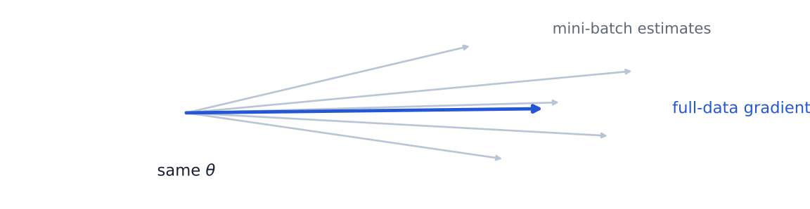
Several gray mini-batch gradient estimates scatter around one blue full-data gradient at the same parameter point.

โˆ‡ฮธLfull=1Nโˆ‘i=1Nโˆ‡ฮธโ„’i,โˆ‡ฮธLฬ‚B=1Bโˆ‘iโˆˆBโˆ‡ฮธโ„’i. \nabla_\theta L_{\mathrm{full}}=\frac1N\sum_{i=1}^{N}\nabla_\theta\mathcal L_i, \qquad \widehat{\nabla_\theta L}_{B}=\frac1B\sum_{i\in B}\nabla_\theta\mathcal L_i.

Smaller batch Larger batch
Noisier estimate More stable estimate
More updates per data pass Fewer updates per data pass
Lower memory requirement Higher memory requirement
Less parallel efficiency Better utilization, up to a limit

Mini-batches trade gradient certainty for computational efficiency and more frequent updates.

The estimate is not an โ€œincorrect gradient.โ€ Its exact variance and unbiasedness depend on the sampling procedure.

Initialization determines what can propagate
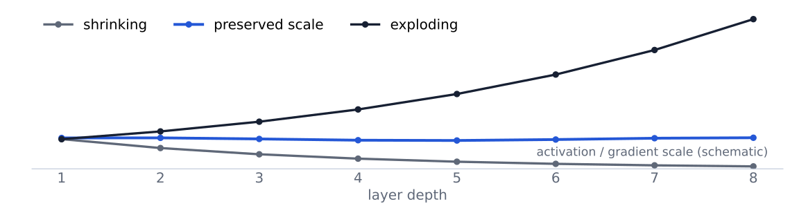
Qualitative layerwise scales shrinking, remaining approximately stable, or exploding across depth.

๐’‰(โ„“โˆ’1)โ†’๐’›(โ„“)โ†’๐’‰(โ„“)\mathbf h^{(\ell-1)}\longrightarrow\mathbf z^{(\ell)}\longrightarrow\mathbf h^{(\ell)}

Varโก(zj(โ„“))โ‰ˆdinVarโก(Wjk(โ„“))Varโก(hk(โ„“โˆ’1)). \operatorname{Var}(z_j^{(\ell)})\approx d_{\mathrm{in}}\operatorname{Var}(W_{jk}^{(\ell)}) \operatorname{Var}(h_k^{(\ell-1)}).

Xavier: Varโก(W)โ‰ˆ2din+dout\text{Xavier: }\operatorname{Var}(W)\approx\frac{2}{d_{\mathrm{in}}+d_{\mathrm{out}}}

He: Varโก(W)โ‰ˆ2dinfor ReLU-like activations\text{He: }\operatorname{Var}(W)\approx\frac{2}{d_{\mathrm{in}}}\quad\text{for ReLU-like activations}

Initialization should keep signals and sensitivities informative across layers.

These variance rules use simplifying assumptions; they do not guarantee stable training in every architecture (Glorot and Bengio 2010; He et al. 2015).

Validation protects the final claim
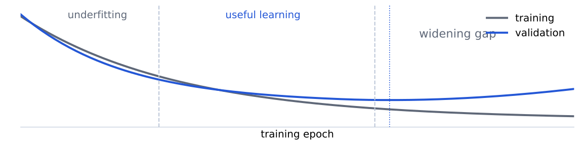
Training loss falls while validation loss reaches a minimum and later rises; regions are labeled underfitting, useful learning, and widening gap.

Split Role
Training Fit model parameters
Validation Select epoch, architecture, and hyperparameters
Test Estimate final performance after decisions are fixed

A decreasing training loss proves successful optimization, not successful generalization.

Early stopping selects an epoch from validation performance. The test set is not monitored as a training curve.

Regularization constrains how the model learns
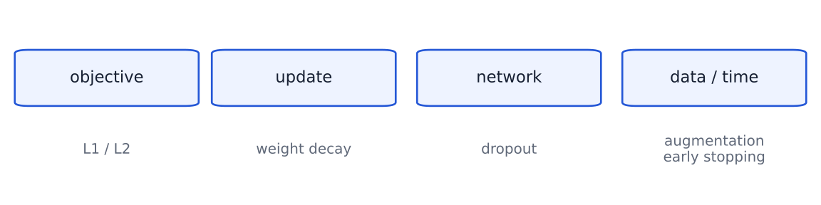
Regularization mechanisms grouped by whether they act on the objective, update, network, data, or training duration.

Mechanism Where it acts Main effect
L1/L2 penalty Objective Discourages parameter configurations
Weight decay Update rule Shrinks selected parameters
Dropout Network during training Randomly masks activations or units during training
Data augmentation Training data Encodes plausible invariances
Early stopping Training duration Limits training-specific adaptation

Regularization constrains parameters, representations, data, or training time.

L2 penalty and weight decay match for ordinary SGD under the corresponding update, but not generally for adaptive optimizers. Dropout is off at evaluation; the framework handles scaling. Biases and normalization parameters are often excluded from weight decay (Srivastava et al. 2014; Loshchilov and Hutter 2019).

A brief history of artificial neural networks

1943 ยท A mathematical neuron

McCulloch and Pitts propose a logical model of neural computation.

1958 ยท A neuron that learns

Rosenblatt introduces the perceptron and its learning rule.

1969 ยท Limits of a single layer

Minsky and Papert analyze what single-layer perceptrons cannot represent.

1970sโ€“1986 ยท Learning through many layers

Reverse differentiation becomes a practical way to assign credit through composed computations.

2006โ€“2012 ยท The deep-learning revival

Better training, larger datasets, GPUs, and new architectures make deep networks practical.

Today ยท Differentiable programming

PyTorch constructs computation graphs and calculates gradients automatically.

Neural networks became transformative when expressive hidden representations met a practical method for assigning credit through many layers.

Person of the day: Geoffrey Hinton

Instructor-provided sketch of Geoffrey Hinton.

Geoffrey Hinton helped turn backward credit assignment into a practical foundation of modern deep learning.

1986 ยท Learning internal representations

Rumelhart, Hinton, and Williams showed how hidden representations can be learned by propagating error derivatives backward (Rumelhart et al. 1986).

2006 ยท Reviving deep networks

Hinton, Osindero, and Teh introduced an influential layer-wise training method for deep belief networks (Hinton et al. 2006).

2012 ยท Deep learning at scale

Krizhevsky, Sutskever, and Hinton demonstrated deep convolutional networks trained with GPUs on ImageNet (Krizhevsky et al. 2012).

โ„’(fฮธ(๐’™),y)โ†’reverse-mode differentiationโˆ‡ฮธโ„’. \mathcal{L}(f_\theta(\mathbf x),y) \quad\xrightarrow{\text{reverse-mode differentiation}}\quad \nabla_\theta \mathcal{L}.

Backpropagation organizes the chain rule through a computation graph. Autograd is the software machinery that performs this differentiation automatically.

2018 ACM Turing Award (Association for Computing Machinery 2019) ยท 2024 Nobel Prize in Physics (Nobel Prize Outreach 2024)

References

Association for Computing Machinery. 2019. โ€œFathers of the Deep Learning Revolution Receive ACM A.M. Turing Award.โ€ https://awards.acm.org/about/2018-turing.
Glorot, Xavier, and Yoshua Bengio. 2010. โ€œUnderstanding the Difficulty of Training Deep Feedforward Neural Networks.โ€ Proceedings of the Thirteenth International Conference on Artificial Intelligence and Statistics, Proceedings of machine learning research, vol. 9: 249โ€“56. https://proceedings.mlr.press/v9/glorot10a.html.
He, Kaiming, Xiangyu Zhang, Shaoqing Ren, and Jian Sun. 2015. โ€œDelving Deep into Rectifiers: Surpassing Human-Level Performance on ImageNet Classification.โ€ Proceedings of the IEEE International Conference on Computer Vision, 1026โ€“34. https://openaccess.thecvf.com/content_iccv_2015/html/He_Delving_Deep_into_ICCV_2015_paper.html.
Hinton, Geoffrey E., Simon Osindero, and Yee-Whye Teh. 2006. โ€œA Fast Learning Algorithm for Deep Belief Nets.โ€ Neural Computation 18 (7): 1527โ€“54. https://doi.org/10.1162/neco.2006.18.7.1527.
Kingma, Diederik P., and Jimmy Ba. 2015. โ€œAdam: A Method for Stochastic Optimization.โ€ International Conference on Learning Representations. https://arxiv.org/abs/1412.6980.
Krizhevsky, Alex, Ilya Sutskever, and Geoffrey E. Hinton. 2012. โ€œImageNet Classification with Deep Convolutional Neural Networks.โ€ Advances in Neural Information Processing Systems 25, 1097โ€“105. https://proceedings.neurips.cc/paper/2012/hash/c399862d3b9d6b76c8436e924a68c45b-Abstract.html.
Loshchilov, Ilya, and Frank Hutter. 2019. โ€œDecoupled Weight Decay Regularization.โ€ International Conference on Learning Representations. https://arxiv.org/abs/1711.05101.
McCulloch, Warren S., and Walter Pitts. 1943. โ€œA Logical Calculus of the Ideas Immanent in Nervous Activity.โ€ The Bulletin of Mathematical Biophysics 5: 115โ€“33. https://doi.org/10.1007/BF02478259.
Minsky, Marvin, and Seymour A. Papert. 1969. Perceptrons: An Introduction to Computational Geometry. The MIT Press. https://mitpress.mit.edu/9780262130431/perceptrons/.
Nobel Prize Outreach. 2024. โ€œThe Nobel Prize in Physics 2024.โ€ https://www.nobelprize.org/prizes/physics/2024/summary/.
PyTorch contributors. n.d.-a. โ€œAutograd Mechanics.โ€ Accessed September 22, 2026. https://docs.pytorch.org/docs/stable/notes/autograd.html.
PyTorch contributors. n.d.-b. โ€œCrossEntropyLoss โ€” PyTorch Documentation.โ€ Accessed September 22, 2026. https://docs.pytorch.org/docs/stable/generated/torch.nn.CrossEntropyLoss.html.
PyTorch contributors. n.d.-c. โ€œLinear โ€” PyTorch Documentation.โ€ Accessed September 22, 2026. https://docs.pytorch.org/docs/stable/generated/torch.nn.Linear.html.
PyTorch contributors. n.d.-d. โ€œtorch.optim โ€” PyTorch Documentation.โ€ Accessed September 22, 2026. https://docs.pytorch.org/docs/stable/optim.html.
PyTorch contributors. n.d.-e. โ€œZeroing Out Gradients in PyTorch.โ€ Accessed September 22, 2026. https://docs.pytorch.org/tutorials/recipes/recipes/zeroing_out_gradients.html.
Rosenblatt, Frank. 1958. โ€œThe Perceptron: A Probabilistic Model for Information Storage and Organization in the Brain.โ€ Psychological Review 65 (6): 386โ€“408. https://doi.org/10.1037/h0042519.
Rumelhart, David E., Geoffrey E. Hinton, and Ronald J. Williams. 1986. โ€œLearning Representations by Back-Propagating Errors.โ€ Nature 323 (6088): 533โ€“36. https://doi.org/10.1038/323533a0.
Srivastava, Nitish, Geoffrey Hinton, Alex Krizhevsky, Ilya Sutskever, and Ruslan Salakhutdinov. 2014. โ€œDropout: A Simple Way to Prevent Neural Networks from Overfitting.โ€ Journal of Machine Learning Research 15 (56): 1929โ€“58. https://www.jmlr.org/papers/v15/srivastava14a.html.
Werbos, Paul John. 1974. โ€œBeyond Regression: New Tools for Prediction and Analysis in the Behavioral Sciences.โ€ PhD thesis, Harvard University. https://www.proquest.com/docview/302768593.

References โ€” continued