Train a latent model
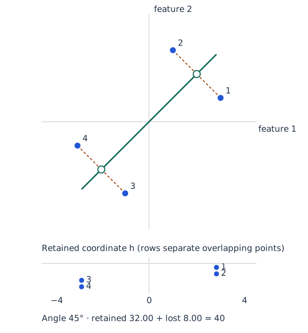
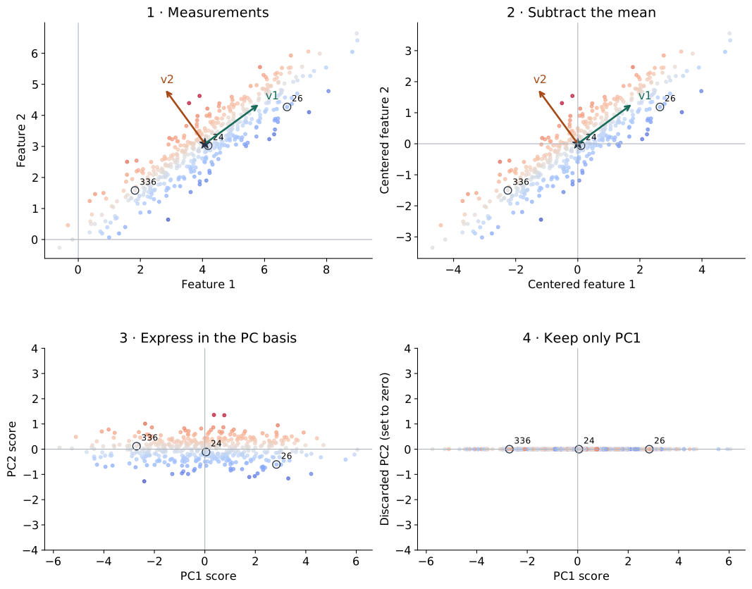
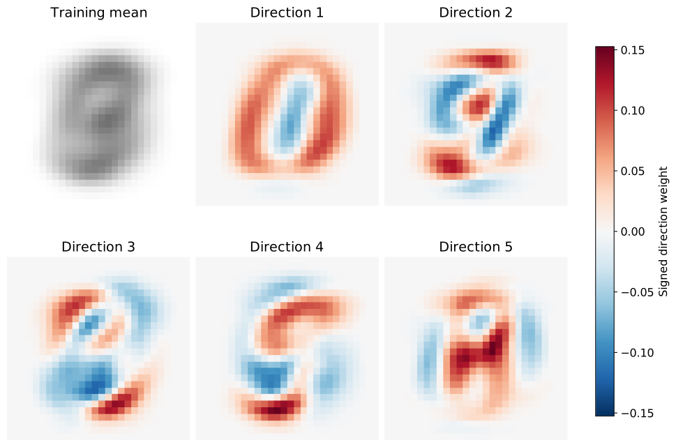
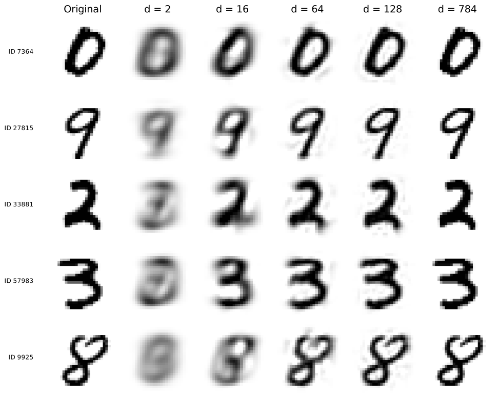
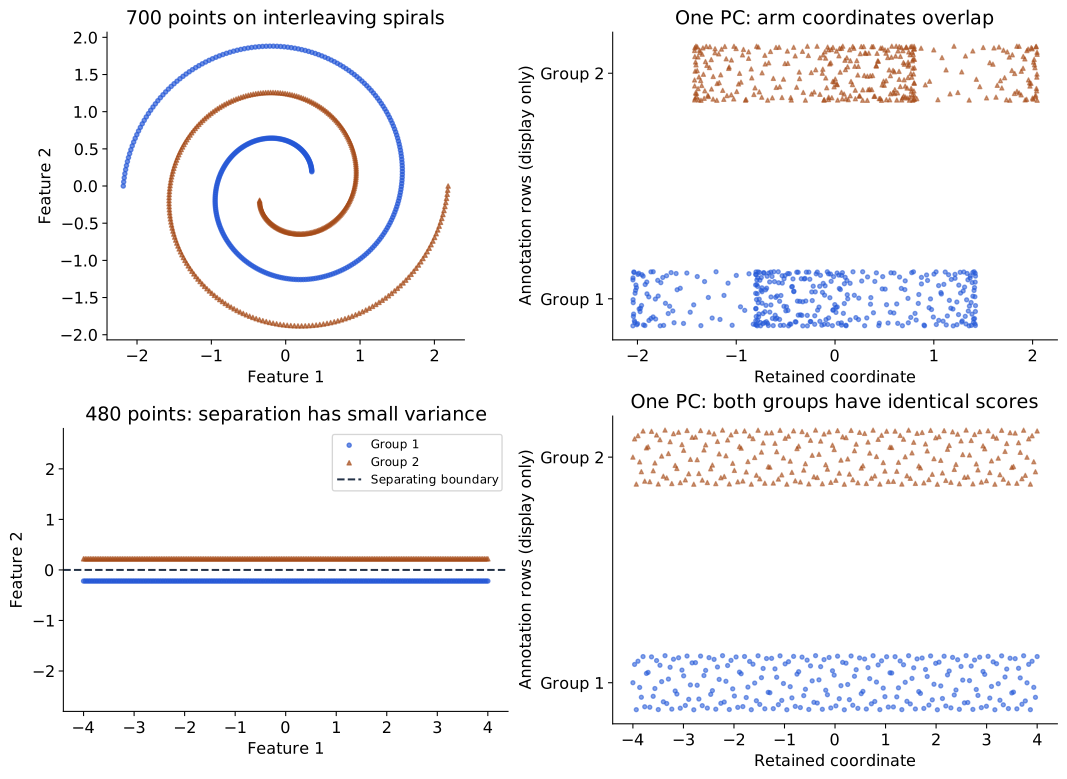
Compress: PCA
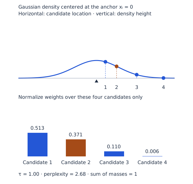
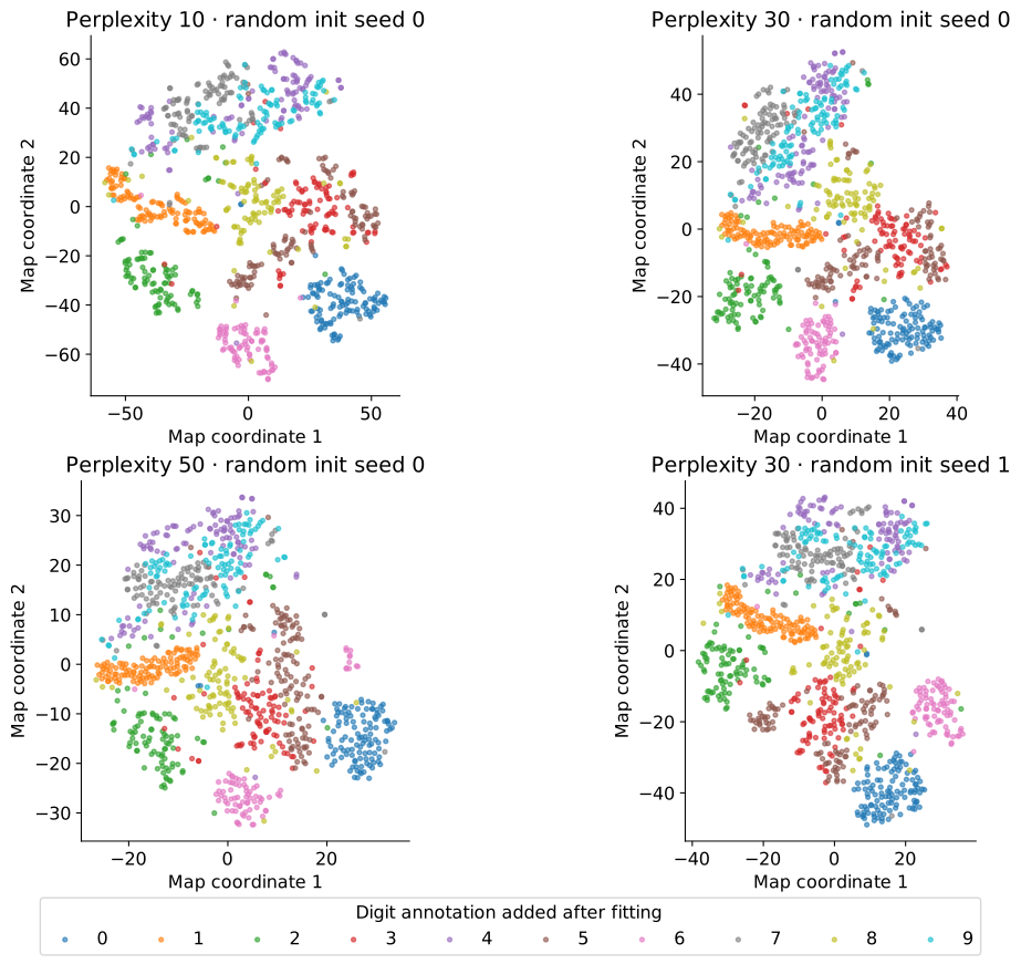
Map: SNE and t-SNE
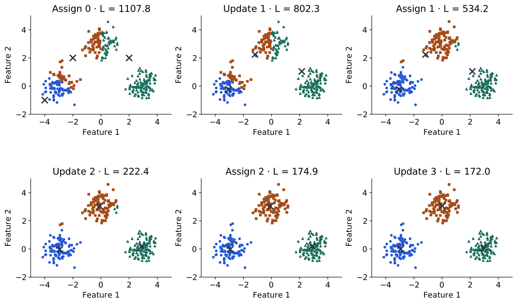
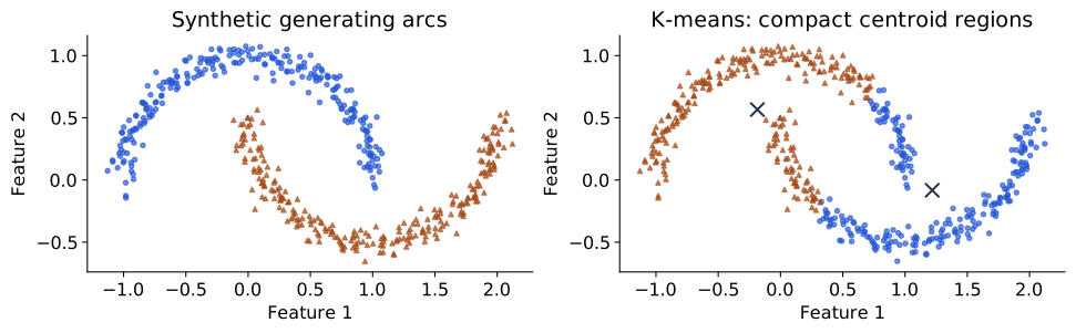
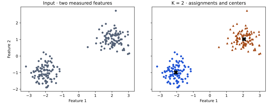
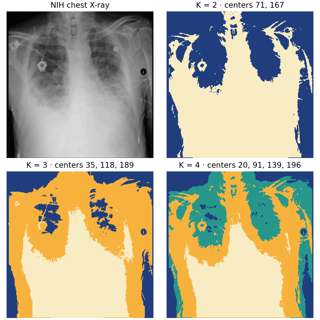
Group: k-means
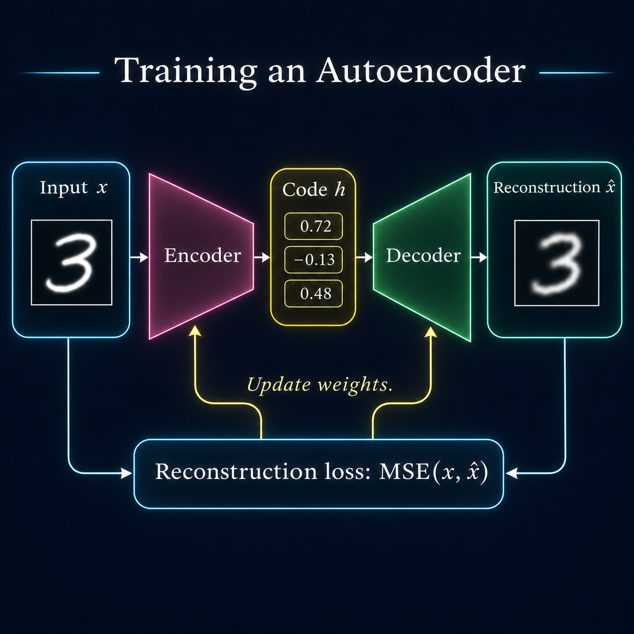
Learn a reconstruction
Train a latent model
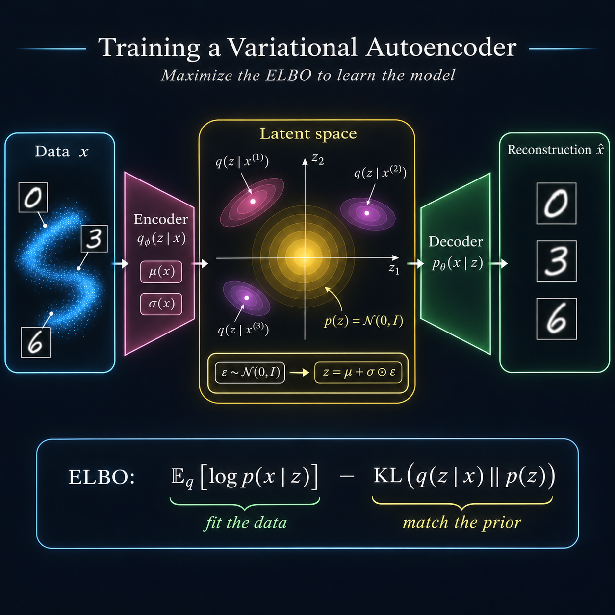
VAE · Learn inference and reconstruction together
The encoder gives each image a distribution of possible codes .
A sampled code enters the decoder; the same input supplies the reconstruction target.
No digit label or correct code is provided.
Follow the chapter order: three distributions; training overview; two jobs; network outputs; derive loss; calculate terms; sample differentiably; train; inspect evidence.
Three distributions, three roles
p ( 𝒛 ) p(\mathbf z) Codes before observing this image?
p θ ( 𝒛 ∣ 𝒙 ) p_\theta(\mathbf z\mid\mathbf x) Which codes explain it under the model?
q ψ ( 𝒛 ∣ 𝒙 ) q_\psi(\mathbf z\mid\mathbf x) What can the encoder approximate?
These describe image codes, rather than network-weight uncertainty.
Fix one image throughout. Before/after refers to observing it, not training epochs. Exact posterior depends on the current decoder and is generally intractable.
From a code to a code distribution
Follow one input to its cloud, one sampled code and reconstruction. Yellow is the fixed prior. Tilted ellipses are conceptual; our encoder covariance is diagonal. Match-prior pressure does not force all posteriors to coincide.
The loss has two jobs
Reconstruction cost: retain information that helps explain this image.
Prior KL cost: compare this image’s approximate posterior with the shared prior.
We will derive why these terms belong together.
Preview only; do not introduce a second derivation. The prior is fixed; image-specific distributions depend on shared encoder weights.
Encoder · Two vectors for every image
𝝁 ( 𝒙 ) , log 𝝈 ( 𝒙 ) ∈ ℝ d . \boldsymbol\mu(\mathbf x),\ \log\boldsymbol\sigma(\mathbf x)\in\mathbb R^d.
𝝈 = exp ( log 𝝈 ) , 𝝈 2 = exp ( 2 log 𝝈 ) . \boldsymbol\sigma=\exp(\log\boldsymbol\sigma),\qquad\boldsymbol\sigma^2=\exp(2\log\boldsymbol\sigma).
q ψ ( 𝒛 ∣ 𝒙 ) = 𝒩 ( 𝒛 ; 𝝁 , diag ( 𝝈 2 ) ) . q_\psi(\mathbf z\mid\mathbf x)=\mathcal N(\mathbf z;\boldsymbol\mu,\operatorname{diag}(\boldsymbol\sigma^2)).
Each batch output has shape ( B , d ) (B,d) 2 d 2d
psi is shared across images; predicted means and spreads depend on the image. These describe code uncertainty, not network weights.
Decoder · Means, then an observation model
g θ ( 𝒛 ) ∈ ℝ D is a vector of pixel means. g_\theta(\mathbf z)\in\mathbb R^D\quad\text{is a vector of pixel means.}
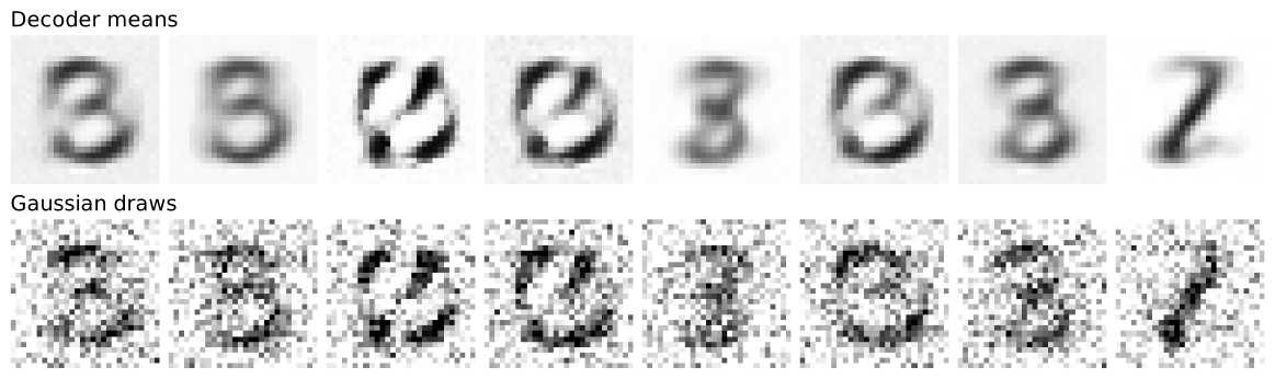
p θ ( 𝒙 ∣ 𝒛 ) = 𝒩 ( 𝒙 ; g θ ( 𝒛 ) , s x 2 𝑰 ) . p_\theta(\mathbf x\mid\mathbf z)=\mathcal N(\mathbf x;g_\theta(\mathbf z),s_x^2\mathbf I).
Evaluating the distribution at an image gives one scalar density.
Latent 𝝈 \boldsymbol\sigma s x s_x
Decoder input is a code. Its neural output is not a single scalar likelihood. Fixed sx shared across pixels; a chosen continuous observation model.
What should training improve?
p θ ( 𝒙 ) = ∫ p θ ( 𝒙 ∣ 𝒛 ) p ( 𝒛 ) d 𝒛 . p_\theta(\mathbf x)=\int p_\theta(\mathbf x\mid\mathbf z)p(\mathbf z)\,d\mathbf z.
We would like to increase log p θ ( 𝒙 ) \log p_\theta(\mathbf x)
The nonlinear decoder makes this integral difficult.
The encoder proposes image-specific codes for a computable bound.
No correct latent-code labels or posterior targets are supplied. Preview the two jobs: explain input and control departures from prior. Derive the bound once in the next slides.
Expose the bound with Bayes’ rule
Fix 𝒙 \mathbf x q ψ ( 𝒛 ∣ 𝒙 ) q_\psi(\mathbf z\mid\mathbf x) D K L ( q ψ ( 𝒛 ∣ 𝒙 ) ∥ p θ ( 𝒛 ∣ 𝒙 ) ) = 𝔼 q ψ ( 𝒛 ∣ 𝒙 ) [ log q ψ ( 𝒛 ∣ 𝒙 ) − log p θ ( 𝒛 ∣ 𝒙 ) ] . \begin{aligned}
D_{\mathrm{KL}}(q_\psi(\mathbf z\mid\mathbf x)\|p_\theta(\mathbf z\mid\mathbf x))\\
=\mathbb E_{q_\psi(\mathbf z\mid\mathbf x)}[\log q_\psi(\mathbf z\mid\mathbf x)-\log p_\theta(\mathbf z\mid\mathbf x)].
\end{aligned}
log p θ ( 𝒛 ∣ 𝒙 ) = log p θ ( 𝒙 ∣ 𝒛 ) + log p ( 𝒛 ) − log p θ ( 𝒙 ) . \log p_\theta(\mathbf z\mid\mathbf x)=\log p_\theta(\mathbf x\mid\mathbf z)+\log p(\mathbf z)-\log p_\theta(\mathbf x).
The posterior comparison is a derivation tool.
Leave board room. Substitute the second equality into the first and group log q minus log prior. Keep the full encoder distribution notation in the KL, expectation and log-density term.
Substitute Bayes and group the terms
For fixed 𝒙 \mathbf x q = q ψ ( 𝒛 ∣ 𝒙 ) q=q_\psi(\mathbf z\mid\mathbf x)
D K L ( q ∥ p θ ( 𝒛 ∣ 𝒙 ) ) = 𝔼 q [ log q − log p ( 𝒛 ) ] − 𝔼 q [ log p θ ( 𝒙 ∣ 𝒛 ) ] + log p θ ( 𝒙 ) . \begin{aligned}
D_{\mathrm{KL}}(q\|p_\theta(\mathbf z\mid\mathbf x))
&=\mathbb E_q[\log q-\log p(\mathbf z)]\\
&\quad-\mathbb E_q[\log p_\theta(\mathbf x\mid\mathbf z)]\\
&\quad+\log p_\theta(\mathbf x).
\end{aligned}
The first expectation is the prior KL .
This missing algebraic step now remains visible. The KL definition is exact; no single-code density comparison replaces its expectation. Log evidence is constant with respect to sampled codes.
Evidence equals bound plus inference gap
ℰ ( 𝒙 ) = 𝔼 q [ log p θ ( 𝒙 ∣ 𝒛 ) ] − D K L ( q ∥ p ( 𝒛 ) ) . \mathcal E(\mathbf x)=\mathbb E_q[\log p_\theta(\mathbf x\mid\mathbf z)]-D_{\mathrm{KL}}(q\|p(\mathbf z)).
log p θ ( 𝒙 ) = ℰ ( 𝒙 ) + D K L ( q ∥ p θ ( 𝒛 ∣ 𝒙 ) ) ⏟ nonnegative gap . \log p_\theta(\mathbf x)=\mathcal E(\mathbf x)+\underbrace{D_{\mathrm{KL}}(q\|p_\theta(\mathbf z\mid\mathbf x))}_{\text{nonnegative gap}}.
Thus ℰ ( 𝒙 ) ≤ log p θ ( 𝒙 ) \mathcal E(\mathbf x)\le\log p_\theta(\mathbf x)
The prior KL belongs in the bound; posterior KL measures its gap.
Name ELBO: evidence lower bound. Exact encoder posterior makes the bound tight for fixed model; it does not require zero prior KL.
Change the sign to get a loss
ℒ ( 𝒙 ) = − ℰ ( 𝒙 ) = 𝔼 q [ − log p θ ( 𝒙 ∣ 𝒛 ) ] ⏟ reconstruction cost + D K L ( q ∥ p ( 𝒛 ) ) ⏟ prior cost . \mathcal L(\mathbf x)=-\mathcal E(\mathbf x)
=\underbrace{\mathbb E_q[-\log p_\theta(\mathbf x\mid\mathbf z)]}_{\text{reconstruction cost}}+\underbrace{D_{\mathrm{KL}}(q\|p(\mathbf z))}_{\text{prior cost}}.
Both networks learn through one objective.
Only these two terms are evaluated or estimated; the posterior gap is not a third penalty. Natural logs give nats per image.
Reconstruction · Multiply pixel densities
For one fixed image and sampled code:
p θ ( 𝒙 ∣ 𝒛 ) = ( 2 π s x 2 ) − D / 2 exp [ − ∥ 𝒙 − g θ ( 𝒛 ) ∥ 2 2 s x 2 ] . p_\theta(\mathbf x\mid\mathbf z)=(2\pi s_x^2)^{-D/2}
\exp\!\left[-\frac{\|\mathbf x-g_\theta(\mathbf z)\|^2}{2s_x^2}\right].
Conditional pixel independence gives a product over pixels .
Negative logarithms turn that product into a sum .
Evaluate each pixel density at its observed value. This is conditional independence given z, not unconditional independence of pixels.
Why squared reconstruction error?
For the fixed Gaussian observation model: NLL ( 𝒙 , 𝒛 ) = ∥ 𝒙 − g θ ( 𝒛 ) ∥ 2 2 s x 2 + D 2 log ( 2 π s x 2 ) . \operatorname{NLL}(\mathbf x,\mathbf z)=\frac{\|\mathbf x-g_\theta(\mathbf z)\|^2}{2s_x^2}+\frac D2\log(2\pi s_x^2).
Pixel-density product → log-density sum.
For each image, estimate the average over encoder codes with one draw during training.
The observation model determines the reconstruction term.
Week07 Bernoulli pixels give BCE; continuous pixels here use Gaussian NLL. Pixel sum differs from latent expectation. Fixed constant can be omitted for gradients but retained when reporting NLL.
Four pixels · Encode, sample, decode
Schematic image: 𝒙 = ( .7 , .4 , .1 , .9 ) \mathbf x=(.7,.4,.1,.9) D = 4 D=4 d = 2 d=2
𝝁 = ( 2 , − 1 ) \boldsymbol\mu=(2,-1) 𝝈 = ( .5 , .2 ) \boldsymbol\sigma=(.5,.2) 𝝐 = ( 1 , − .5 ) \boldsymbol\epsilon=(1,-.5)
𝒛 = 𝝁 + 𝝈 ⊙ 𝝐 = ( 2.5 , − 1.1 ) . \mathbf z=\boldsymbol\mu+\boldsymbol\sigma\odot\boldsymbol\epsilon=(2.5,-1.1).
Suppose g θ ( 𝒛 ) = ( .8 , .2 , .2 , .8 ) g_\theta(\mathbf z)=(.8,.2,.2,.8) s x = .25 s_x=.25
These are illustrative outputs, not measurements. Introduce shift-and-scale sampling here as the operation used; explain its gradient mechanism later in the chapter sequence.
Four pixels · Score the original image
1
.7
.8
.08
2
.4
.2
.32
3
.1
.2
.08
4
.9
.8
.08
NLL = .56 + C \operatorname{NLL}=.56+C C = 2 log ( 2 π s x 2 ) C=2\log(2\pi s_x^2)
Each row divides the squared residual by 2 times .25². Product of four densities gives sum of their negative logs. One whole-image cost for one code; changing code changes the cost.
Prior KL · Use the Gaussian formula
The encoder gives a diagonal Gaussian with means μ k \mu_k σ k \sigma_k
D K L ( q ψ ( 𝒛 ∣ 𝒙 ) ∥ p ( 𝒛 ) ) = 1 2 ∑ k = 1 d [ μ k 2 + σ k 2 − 1 − 2 log σ k ] .
D_{\mathrm{KL}}\!\left(q_\psi(\mathbf z\mid\mathbf x)\,\|\,p(\mathbf z)\right)
=\frac12\sum_{k=1}^d
\left[\mu_k^2+\sigma_k^2-1-2\log\sigma_k\right].
Compute this directly from the encoder outputs. It penalizes means away from zero and variances away from one.
Why neither term works alone
Reconstruction alone: no explicit prior cost for distant, extremely narrow image-specific code distributions.
KL alone: every image could receive the same standard normal and pay zero.
Together, the terms balance image information and prior cost.
An image of a 3 must retain its strokes. Low KL alone is not evidence of good representation; reconstruction alone is not a sampling model. Do not claim every posterior should equal the prior.
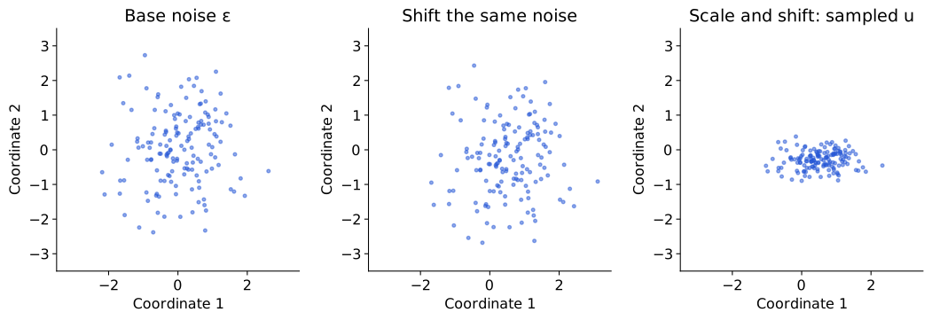
Shift and stretch fixed noise
Hold the noise fixed while differentiating one pass; fresh noise later. Both encoder heads get reconstruction gradients. Halve log variance before exponentiation if translating that parameterization.
Algorithm · One VAE training step
Encode: predict 𝝁 \boldsymbol\mu log 𝝈 \log\boldsymbol\sigma Sample: 𝒛 = 𝝁 + exp ( log 𝝈 ) ⊙ 𝝐 \mathbf z=\boldsymbol\mu+\exp(\log\boldsymbol\sigma)\odot\boldsymbol\epsilon Reconstruct: decode 𝒛 \mathbf z Score: add NLL and prior KL; average over the batch.Update: backpropagate; update both networks; repeat.
Sum pixel and latent contributions within each image.
Return mentally to Figure 22: encoder heads, noise path, decoder, two objective terms. Prior fixed. One fresh noise draw per image. Weights shared; no separately stored training code optimized.
Batch loss · Average the per-image costs
For image i i 𝒛 i \mathbf z_i q ψ ( ⋅ ∣ 𝒙 i ) q_\psi(\cdot\mid\mathbf x_i)
R i = − log p θ ( 𝒙 i ∣ 𝒛 i ) , K i = D K L ( q ψ ( ⋅ ∣ 𝒙 i ) ∥ p ) .
R_i=-\log p_\theta(\mathbf x_i\mid\mathbf z_i),\qquad
K_i=D_{\mathrm{KL}}\!\left(q_\psi(\cdot\mid\mathbf x_i)\,\|\,p\right).
ℒ ̂ b a t c h = 1 B ∑ i = 1 B ( R i + K i ) . \widehat{\mathcal L}_{\mathrm{batch}}=\frac1B\sum_{i=1}^B(R_i+K_i).
Sum over pixels in R i R_i K i K_i
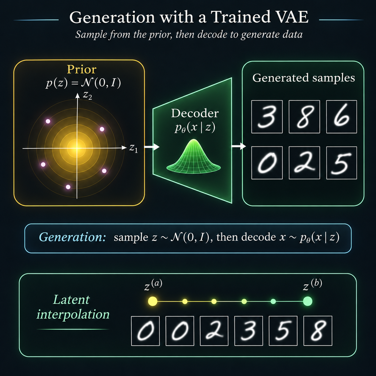
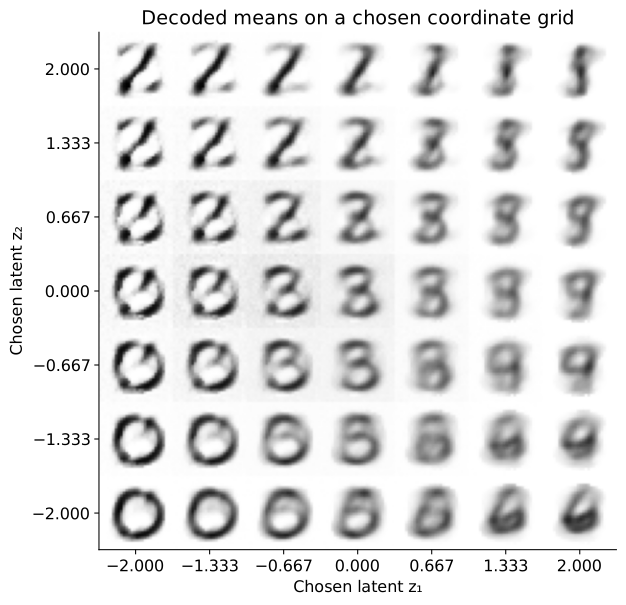
Generation and interpolation
How would you choose a method tomorrow?
PCA: saved linear coordinates. t-SNE: inspect neighbors.
K-means: compact groups.
AE: nonlinear reconstruction. VAE: latent probabilistic learning.
Next: construct training relationships for useful representations.
Week11 self-supervised learning revisits where targets come from and downstream evaluation. These methods are alternatives for purposes, not a compulsory pipeline.
Questions that changed the picture
2006: learned low-dimensional reconstruction — Hinton & Salakhutdinov.
2008: local-affinity maps — van der Maaten & Hinton.
2013/2014: joint latent generation and inference — Kingma & Welling.
History connects methods to the problems they addressed.
2006 paper is not the invention of all autoencoders. AEVB: 2013 preprint, ICLR2014. Credit collaborators; no citation-count ranking.
People of the day: Kingma and Hinton
Diederik P. (Durk) Kingma
Variational autoencoders with Max Welling .
Geoffrey Hinton
Autoencoders with Ruslan Salakhutdinov ; t-SNE with van der Maaten .
References: geometry, grouping and maps
References: learned latent representations