From time-series tasks
to learned representations
and foundation models.
Lecture 2 · 90 minutes

From time-series tasks
to learned representations
and foundation models.
Lecture 2 · 90 minutes
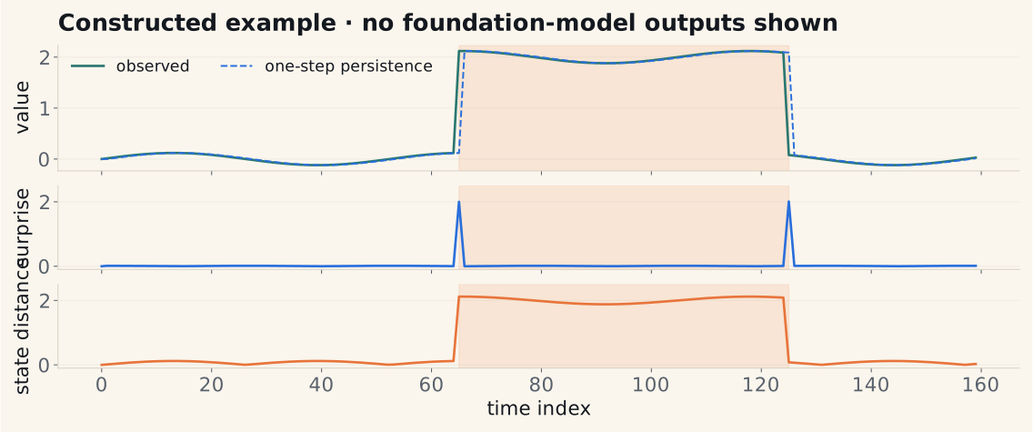
It predicts the next reading accurately.
Does that prove normal operation?
Keep this question open until the final experiment.

Choose the required output before choosing the model.
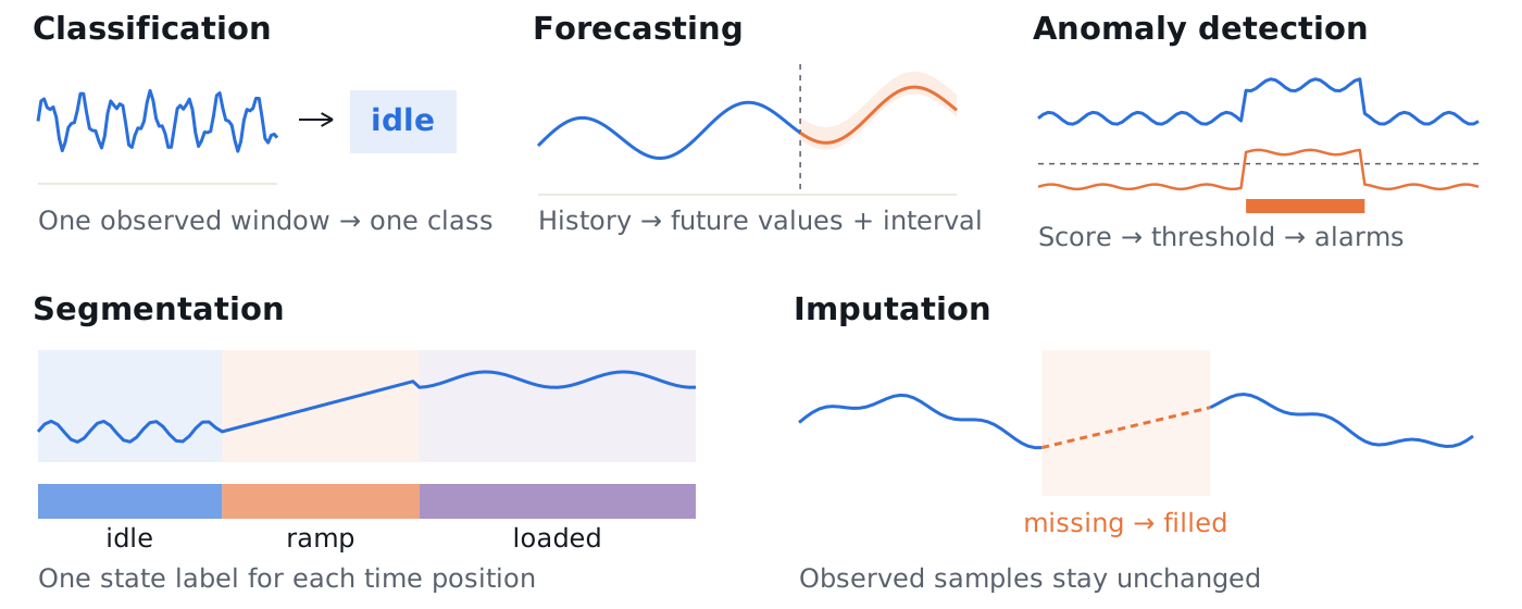
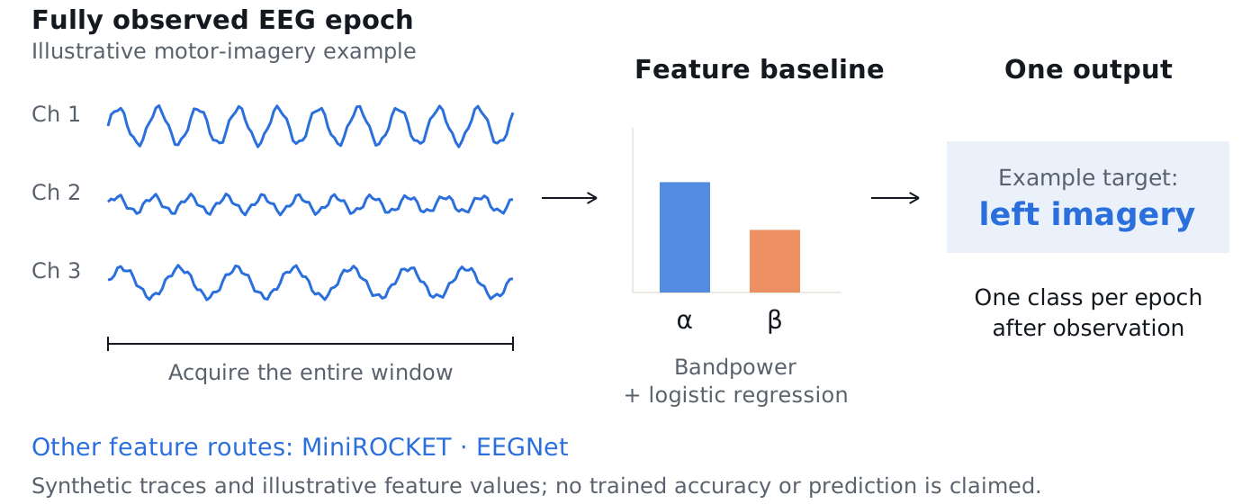
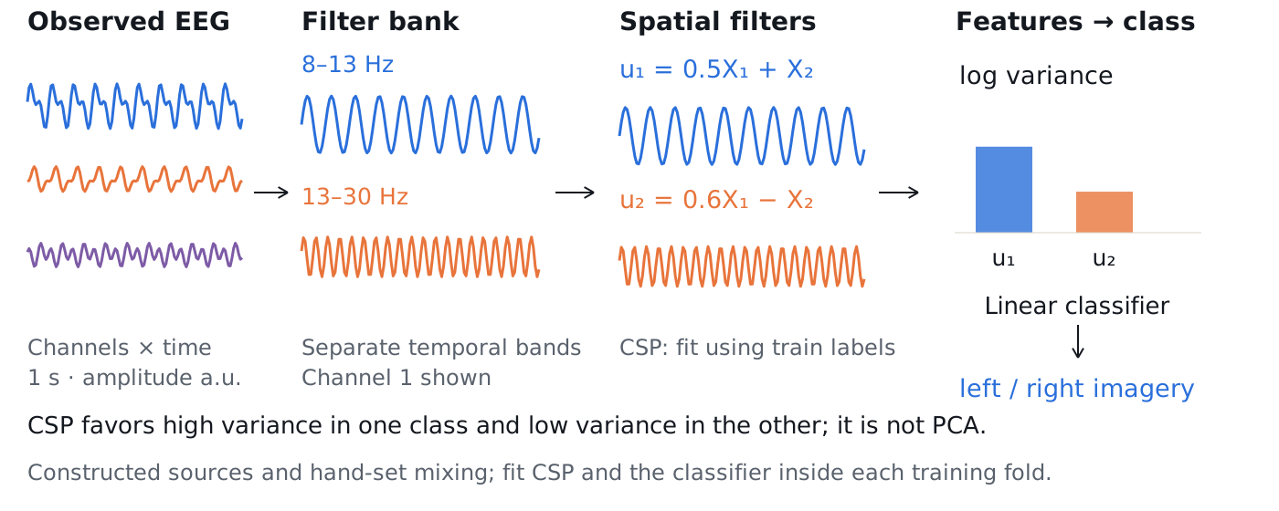
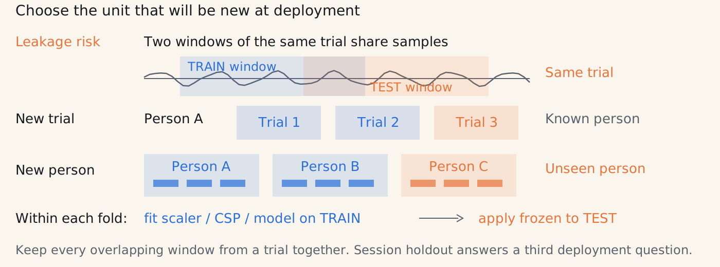
One observed epoch → one class. Bandpower + logistic regression; MiniROCKET features or learned EEGNet features.
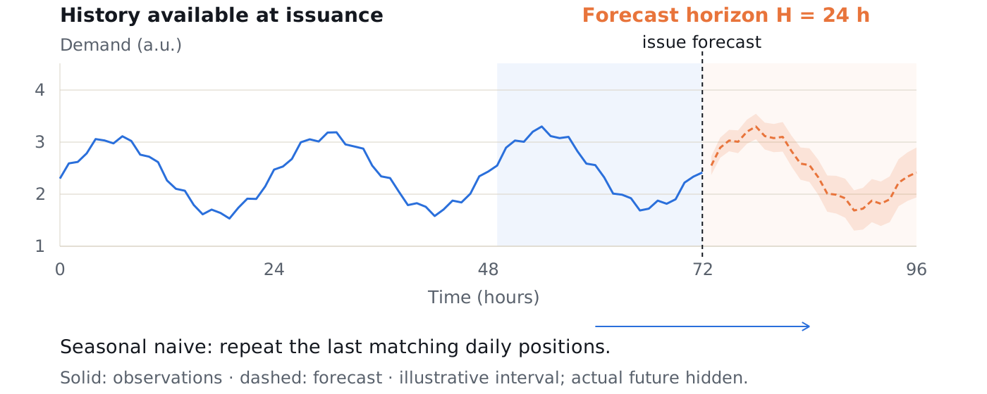
History → future horizon. Compare every model at the same issuance time and forecast horizon.
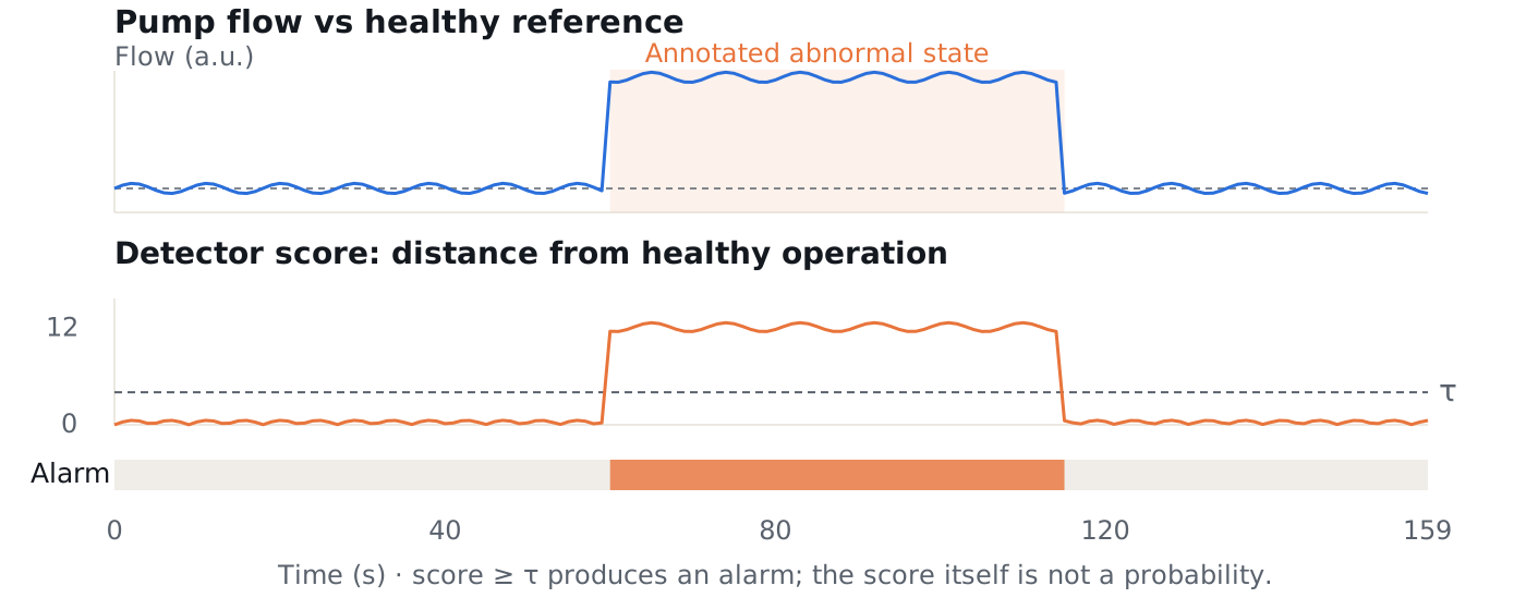
A score becomes a decision only after thresholding. Define whether the label covers an onset or the entire abnormal state.
State labeling: HMM or temporal CNN. Change-point detection: PELT / ruptures.
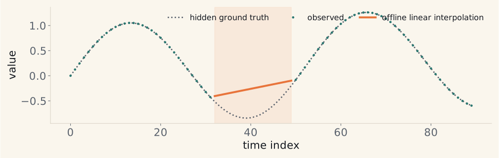
Linear interpolation → Kalman methods → SAITS. Offline filling may use right context; online filling may not.
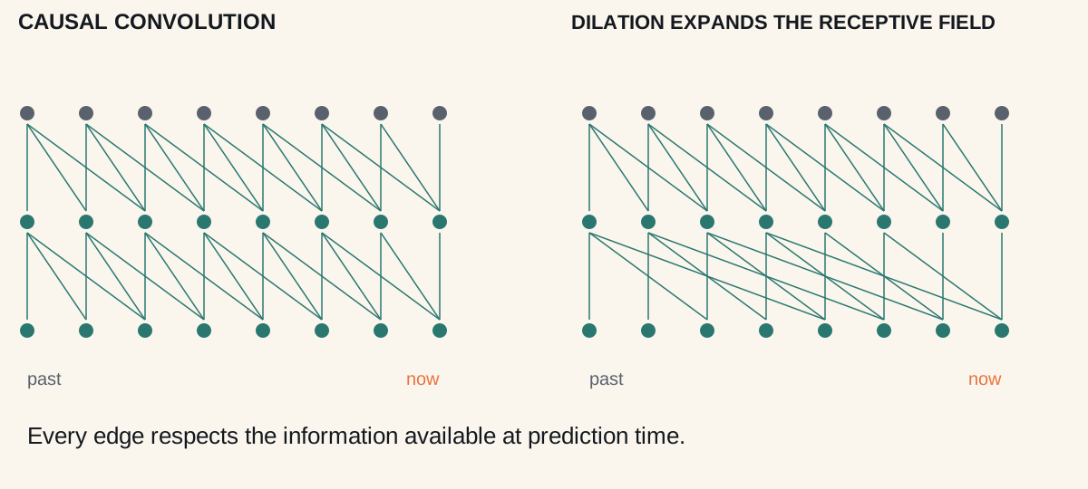
Dilation skips input positions while retaining a local kernel. Future values must stay outside the receptive field.
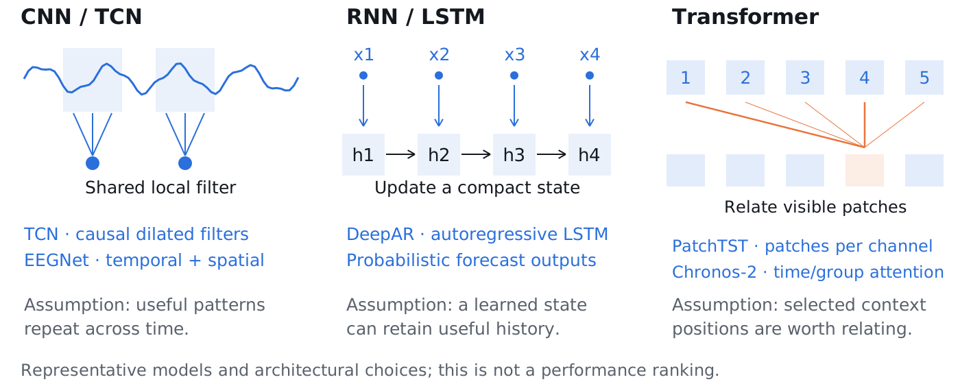
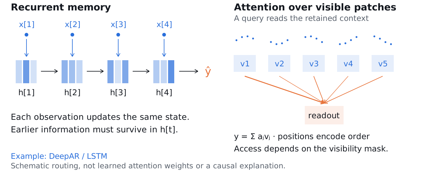
Both can learn long dependencies; they store and access the available history differently.
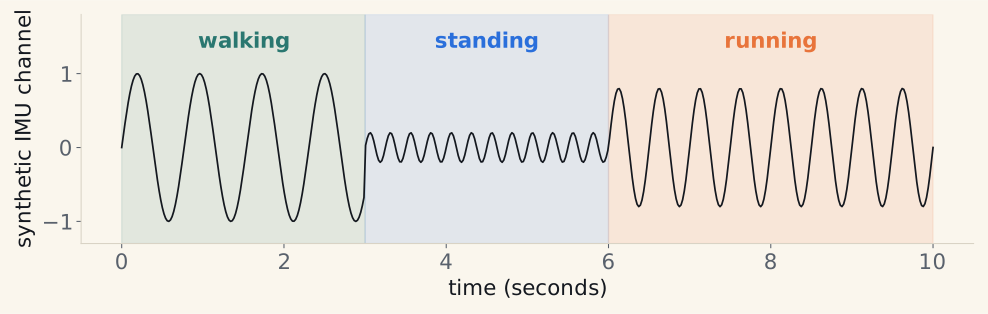
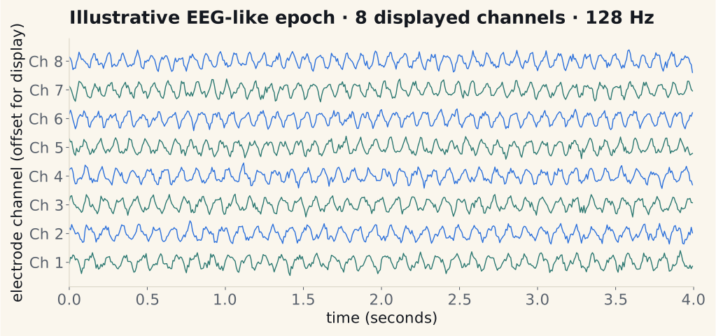
Same axis-reading skill, different target: one movement label for an observed EEG epoch.
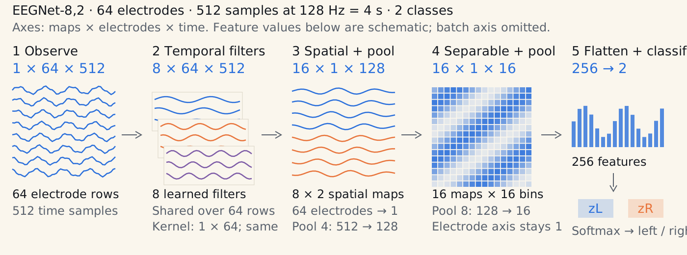
EEGNet makes a related sequence of temporal and spatial operations learnable end to end.
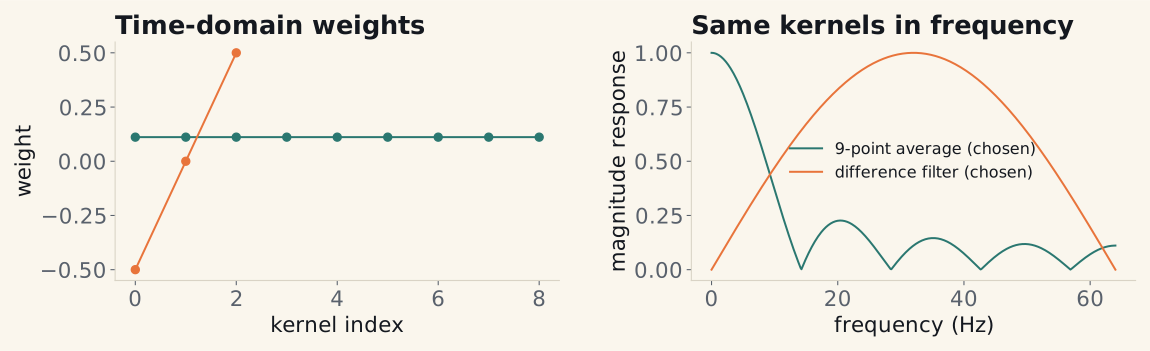
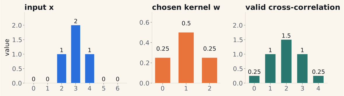
These kernels are chosen by hand. EEGNet learns temporal weights; we can inspect them with the same Fourier tools.
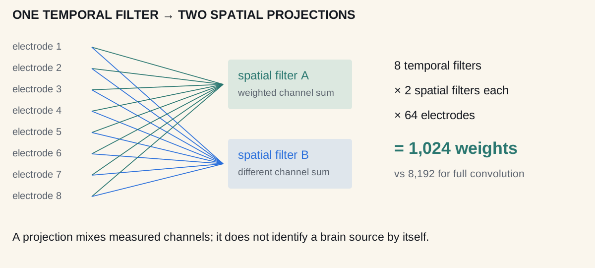
Each temporal feature gets its own spatial projections. Depthwise means we do not mix different temporal filters here.
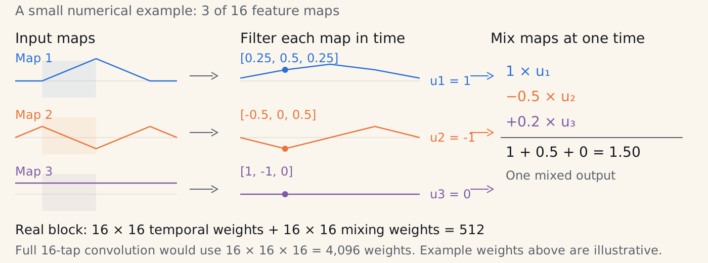
Focus: Distinguish per-map temporal refinement from pointwise feature-map mixing.
Focus: Follow which EEGNet operations change maps, electrodes and time.
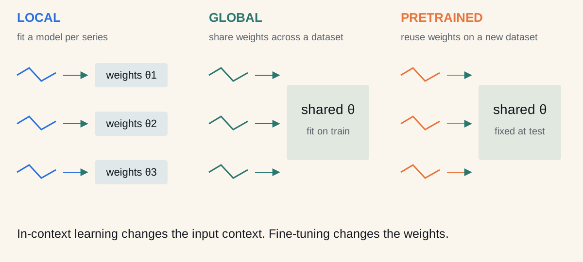
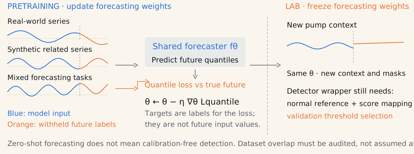
Local models fit each series. Global models share weights. A pretrained forecaster reuses weights on a new task.
autogluon/chronos-2-small · 6 blocks · 8 heads · hidden size 512 · 13 quantiles
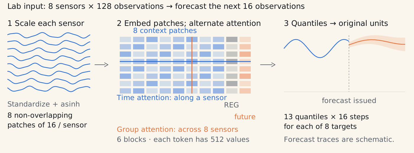
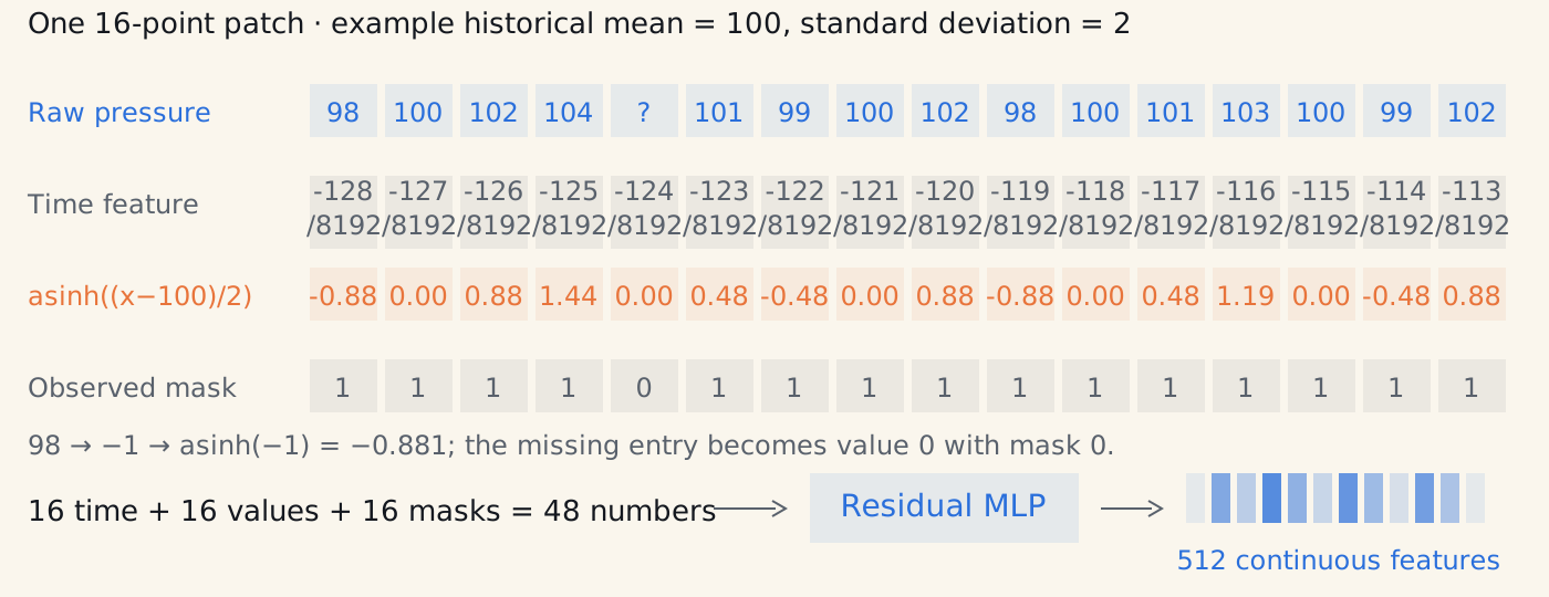
z = asinh((x − μ) / σ) → x̂ = μ + σ sinh(ẑ)
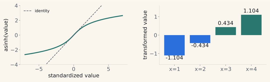
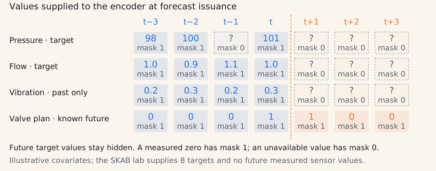
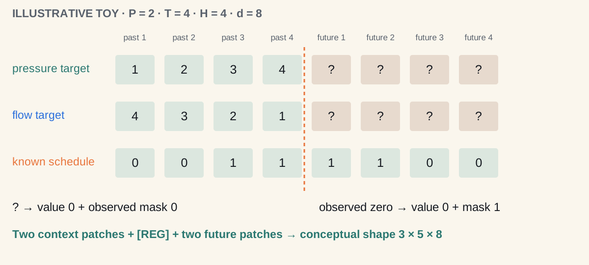
The schedule is hypothetical. These are input-construction numbers, not a measured forecast.
Focus: Explain how values, time and an observation mask become one patch representation.
Chronos-2 uses an encoder. Its time attention is bidirectional across the supplied context and future placeholders.
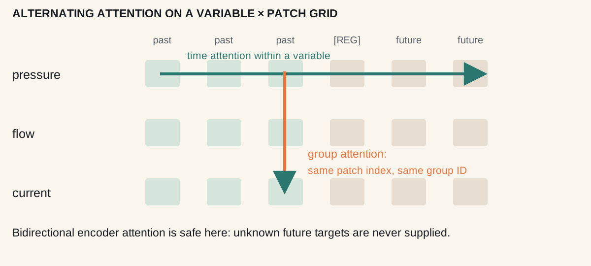
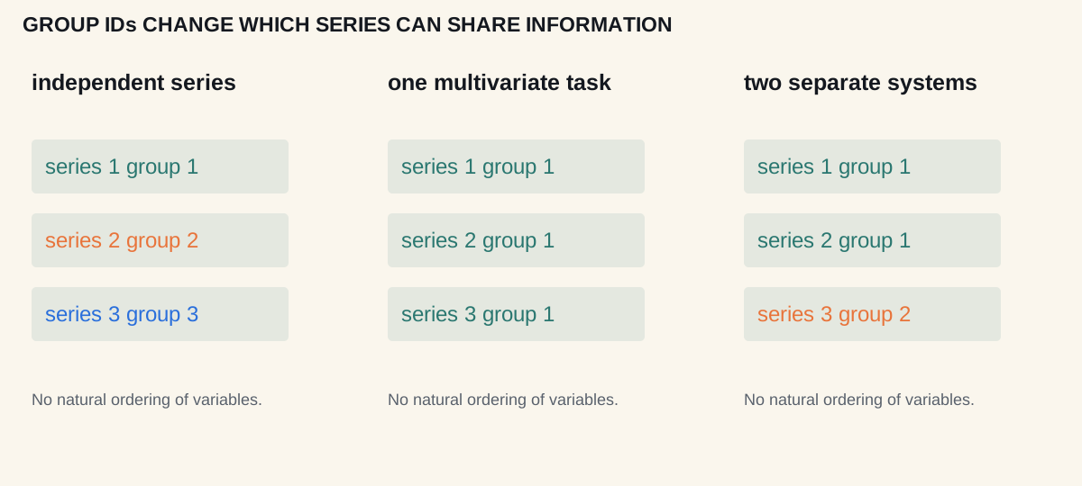
At one patch index, series with the same group ID exchange information. Different group IDs block that exchange.
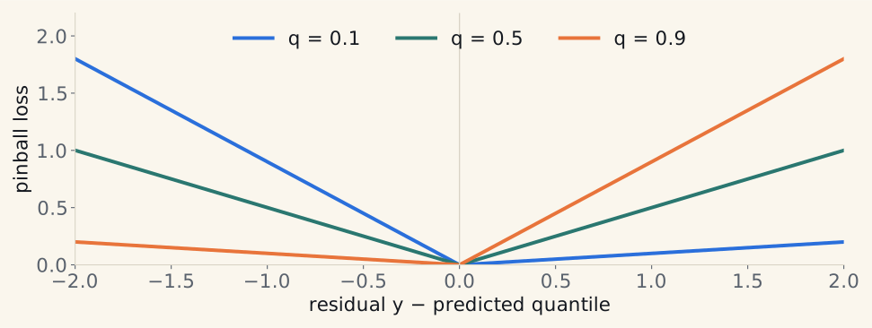
At q = 0.9: underpredict by 1 → loss 0.9; overpredict by 1 → loss 0.1.
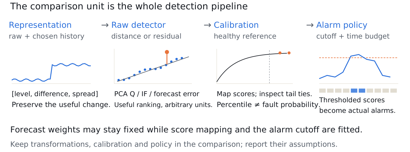
Compare complete detection systems, then inspect which stage explains their differences.
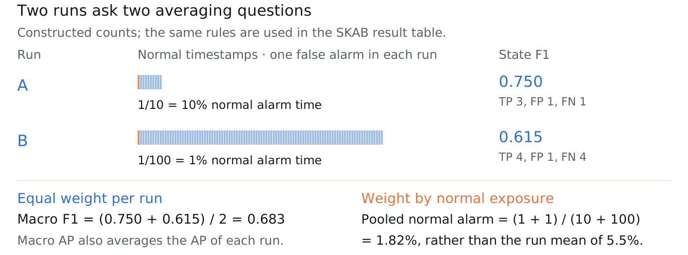
In this lab, AP and F1 give every run one vote; normal alarm time gives every normal timestamp one vote.
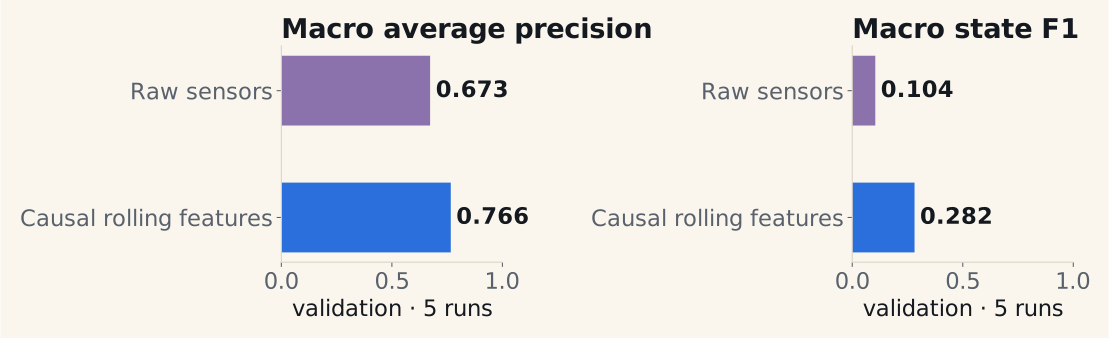
Same Isolation Forest: 200 trees. Raw sensors → 48 causal sensor, difference and rolling features. Validation only.
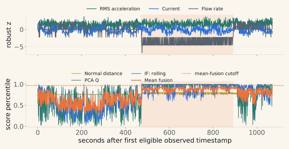
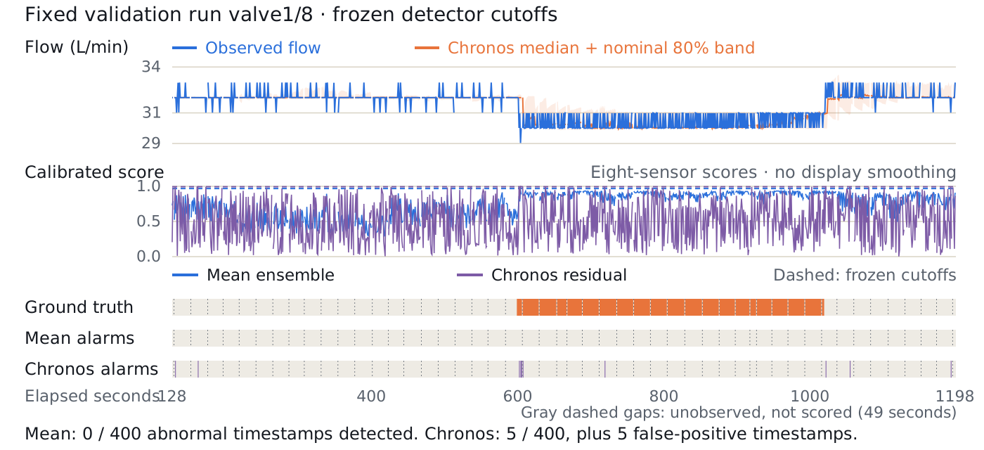
Fixed validation run: valve1/8. Shading = abnormal state. Mean fusion averages three calibrated scores.
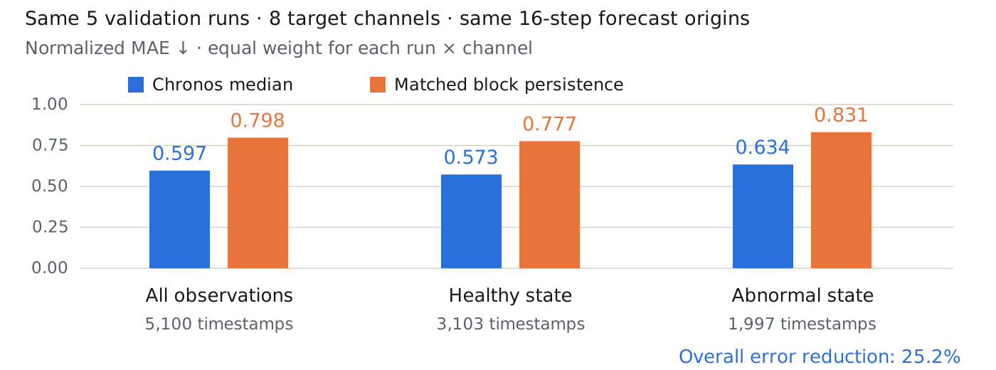
Chronos reduces point-forecast error on these validation runs; its selected residual detector still misses most faulty timestamps.
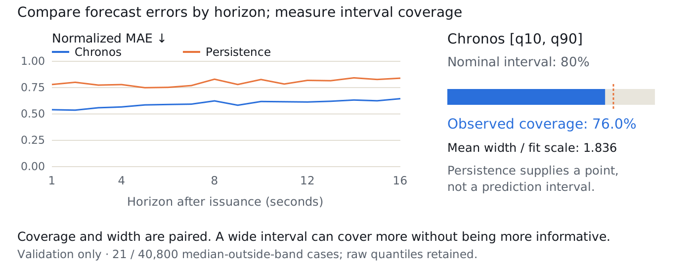
The nominal 80% Chronos interval covers about 76% here. Read coverage together with width.
A high score is not an alarm. On this fixed run, the mean ensemble issues no alerts at its frozen cutoff.
Specify the target.
Follow the axes and the masks.
Compare with an honest baseline.
In the lab: explain one success and one failure before changing the model.

← / → or Space: next scene step, then next slide
Shift + ← / →: skip directly to another slide · Home / End: first / last
E: Lecture / Explore · R: restart the current scene or transfer check
O: overview · A: pen · C: clear · F: fullscreen
Transfer checks: choose, explain, then reveal. Right reveals reasoning after choosing and explaining. Shift+arrows skips slides.
Esc: close panel · #: slide number in the URL
Print / Save as PDF: slides plus selected scene keyframes. Annotations stay in this browser tab.