Lecture 1 · Listening to Time

Core idea

Would you keep this pump running?

Choose measurements and features that keep the intended fault visible.

One reading looks normal.
The recent history may tell another story.

Intro to ML · Two lectures + a practical lab

Serega, the recurring illustrated guide, points toward the problem.

Signals in the world

Core idea

Time changes the question

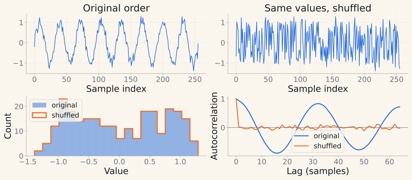
The order, spacing, and context of observations carry information.

A robot

IMU and joint currents

Is it moving normally?
What happens next?

A person

EEG and heart activity

Which state or event produced this epoch?

A service

Requests, latency, energy

Is this spike a fault, a daily pattern, or growth?

Our lab case · SKAB

Worked example

One physical system, eight channels

A water-circulation testbed links motor, hydraulic, thermal, and vibration summaries.

The operational target

Core idea

Keep the whole abnormal state visible

State detection: keep flagging the interval. Onset: mark when it begins.

Three real SKAB channels aligned in time; the provided anomalous-state label is shaded. — Real SKAB valve1/1.csv · orange = provided anomalous-state label · no model predictions

The observation contract

Core idea

An observation is more than a number

Timestamp
when?→Value + unit
what quantity?→Channel + quality
where? trustworthy?

X ∈ ℝ^{T × C}

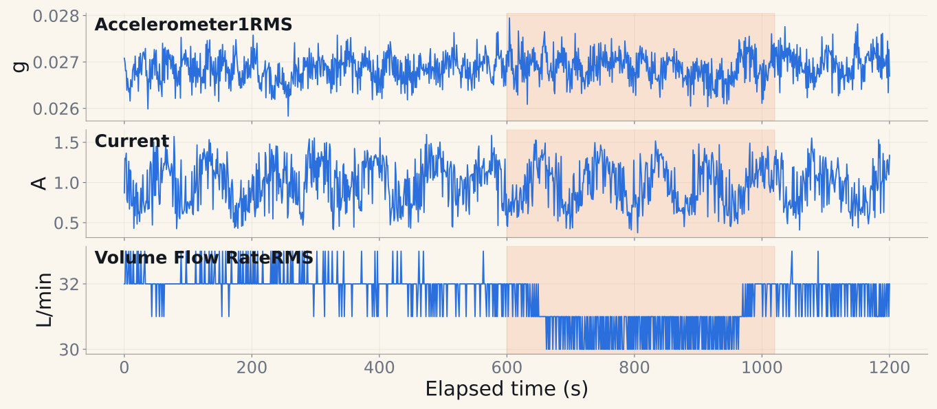
A row is a synchronized observation, not an independent example.

Core idea

What does one row mean?

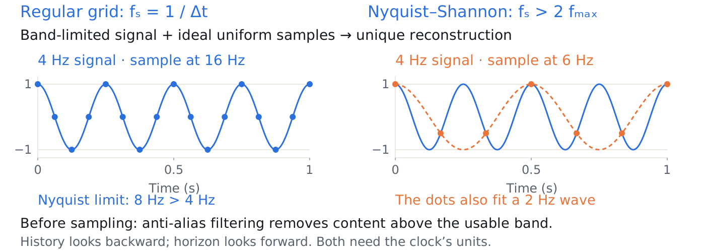
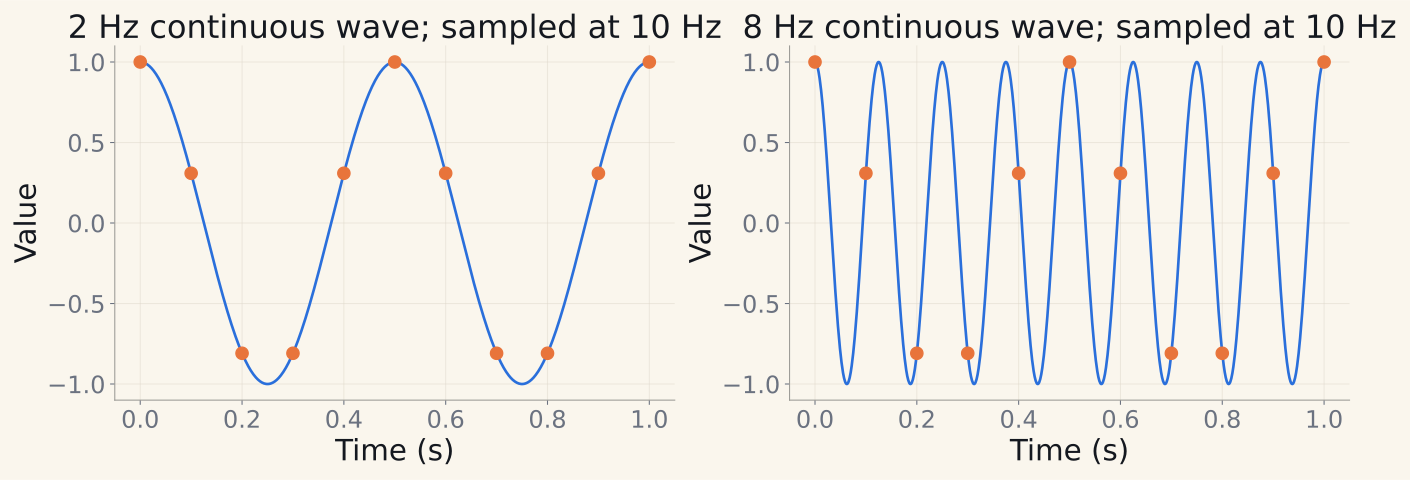
The clock sets units; the sampling rule sets which frequencies can be recovered.

The same 4 Hz cosine is sampled above and below its Nyquist requirement; the undersampled points also fit 2 Hz.

Inspect the real clock

Worked example

One row is not always one second

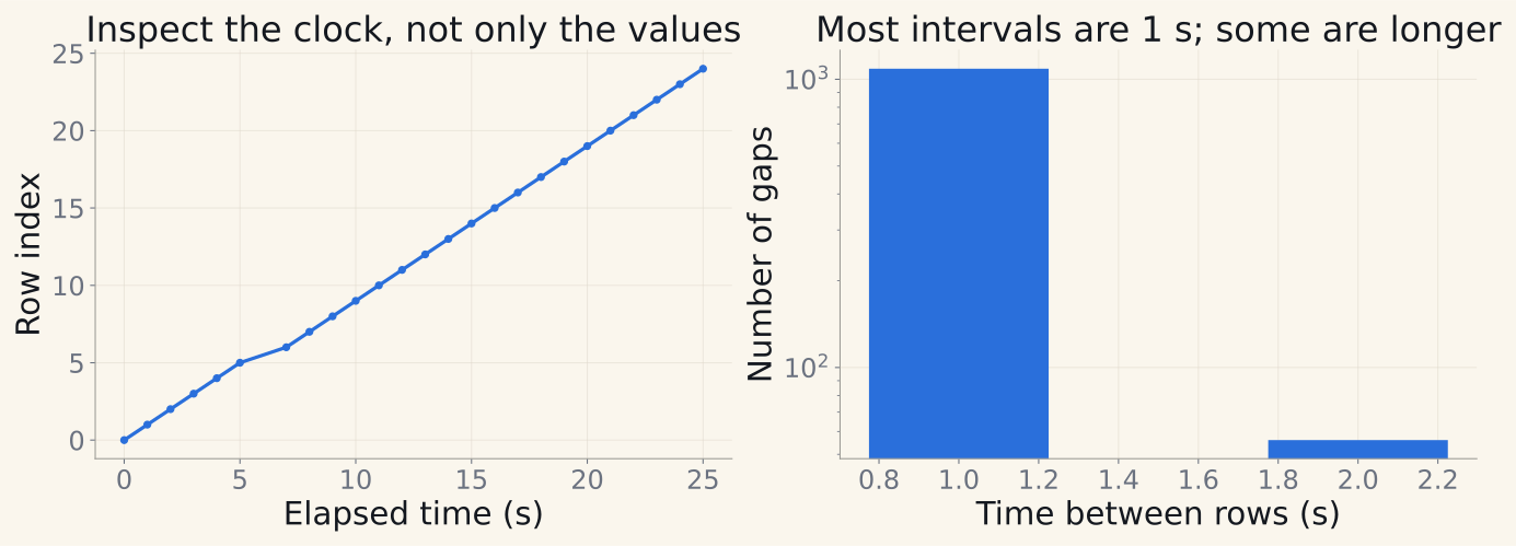
Regularize deliberately. Keep an observation mask; fill only by a declared causal rule.

A SKAB timestamp gap diagnostic: row index versus elapsed time and a histogram of gap durations. — Real SKAB valve1/1.csv · inspect Δt before resampling

A summary is not the waveform

Core idea

What did RMS erase?

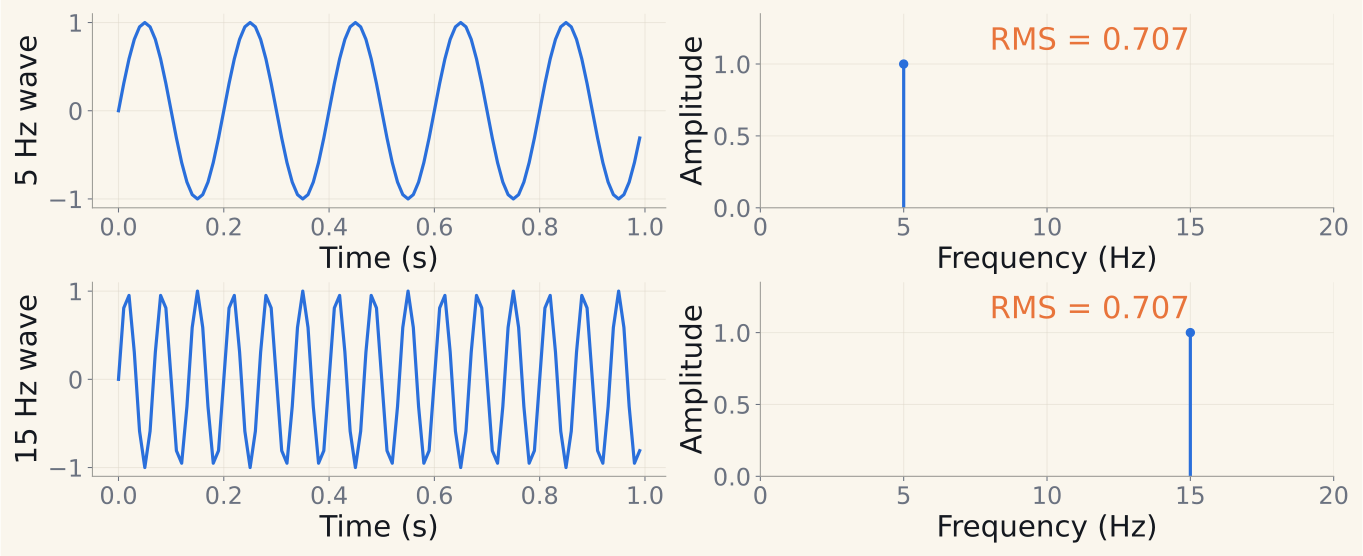
Same energy summary. Different oscillation frequencies. RMS cannot recover the original vibration spectrum.

Synthetic 5 Hz and 15 Hz sinusoids have different spectra but the same RMS of about 0.707. — Constructed teaching signal · fixed seed 20261029

Control the representation

Worked example

Same values. A different story.

Original periodic sequence and its shuffled values: identical histograms, different autocorrelation. — Constructed teaching signal · fixed seed 20261029

Pump investigation 1/8 · Does the pump repeat itself?

Worked example

How far does memory reach?

Lag scatterplots at 1, 8 and 16 samples for the same constructed periodic signal. — Constructed teaching signal · fixed seed 20261029

Change one component at a time

Worked example

Trend, seasonality, and residuals

For this teaching signal: x[t] = trend[t] + seasonal[t] + noise[t].

A constructed time series with a known linear trend, 32-sample seasonal wave, and noise. — Constructed teaching signal · fixed seed 20261029

Pump investigation 2/8 · What changed in the readings?

Worked example

A flat mean can hide a change

The noise scale increases halfway through a constructed series; rolling standard deviation changes more clearly than rolling mean. — Constructed teaching signal · fixed seed 20261029

Stable with respect to what?

Core idea

Stationarity is an assumption to inspect

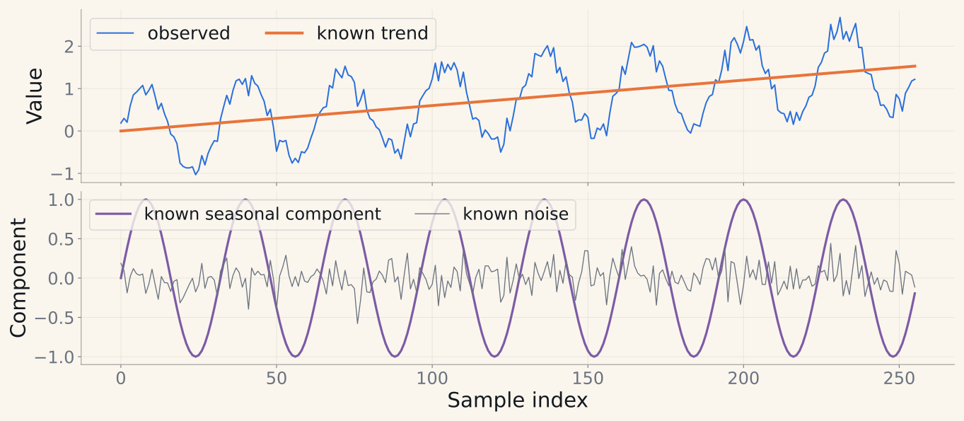
Focus: Treat stationarity as a modelling assumption that requires evidence.

Weak stationarity

Constant mean and finite variance

Autocovariance depends on lag, not absolute time

Useful diagnostics

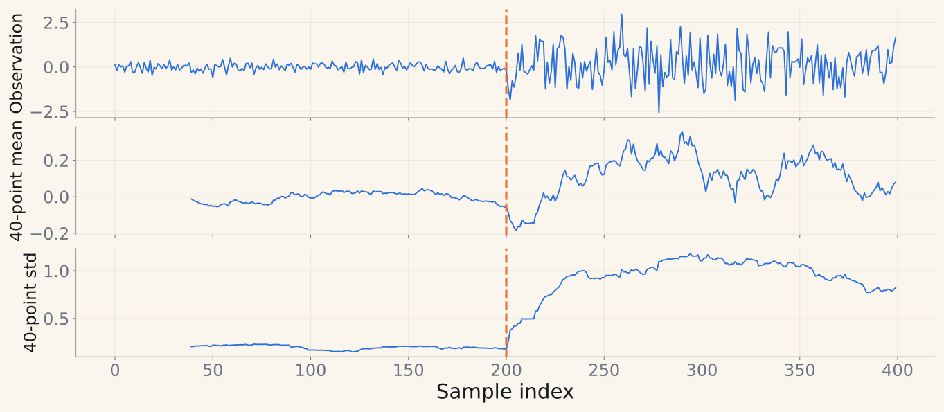
Compare local means and spreads

Inspect ACF, regimes, and residuals

A flat plot or one statistical test cannot establish every assumption.

A compact diagnostic map

Reference detail

What else can change?

Property	Measure or plot	What it can reveal
Level / scale	Median, MAD, quantiles	Offsets, amplitude changes
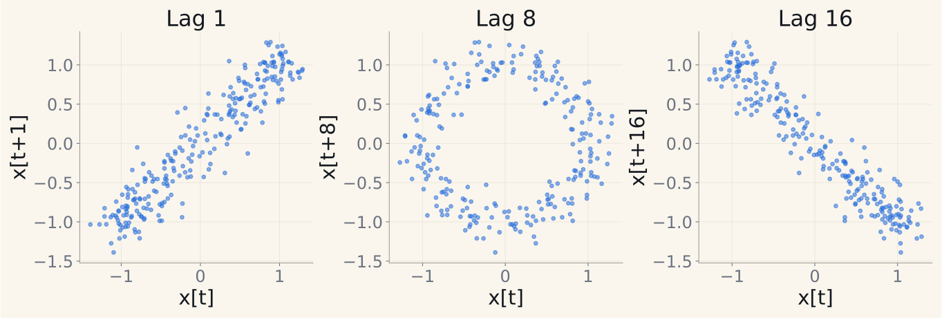
Dependence	ACF, lag and channel plots	Memory, changed relationships
Observation quality	Gap lengths, masks, saturation	Sensor and logging failures
Local dynamics	Differences, local slope, spectrum	Transitions, oscillation changes

Return to the pump

Core idea

Normal depends on the operating regime

A current value may be normal during startup and unusual at steady speed.

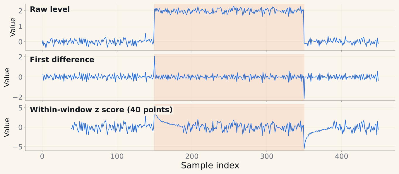
A new level may be a fault, a commanded change, or a new operating mode.

Labels and the monitoring goal give “unusual” its meaning.

Serega wonders which operating regime should count as normal.

Time · frequency · time–frequency

Core idea

One signal, three coordinate views

Explain what a representation preserves, loses and locates in time.

Time

What happened, and when?

Waveform, lags, local statistics

Frequency

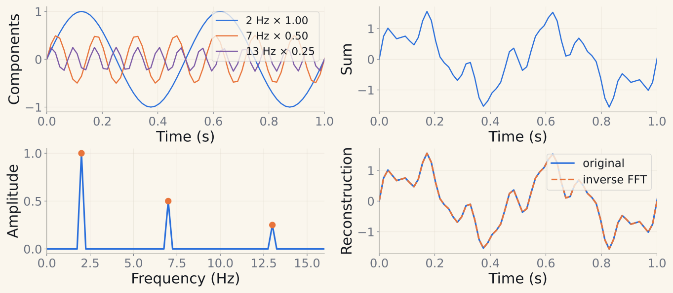
Which rhythms are present?

Fourier coefficients, magnitude, power

Time–frequency

When did each rhythm appear?

STFT spectrogram, wavelet scalogram

Pump investigation 3/8 · Which rhythms are present?

Worked example

Build a signal from simple waves

Three known frequency components, their sum, the exact amplitude peaks, and reconstruction by inverse FFT. — Constructed teaching signal · fixed seed 20261029

Worked example

A repeated shape creates harmonics

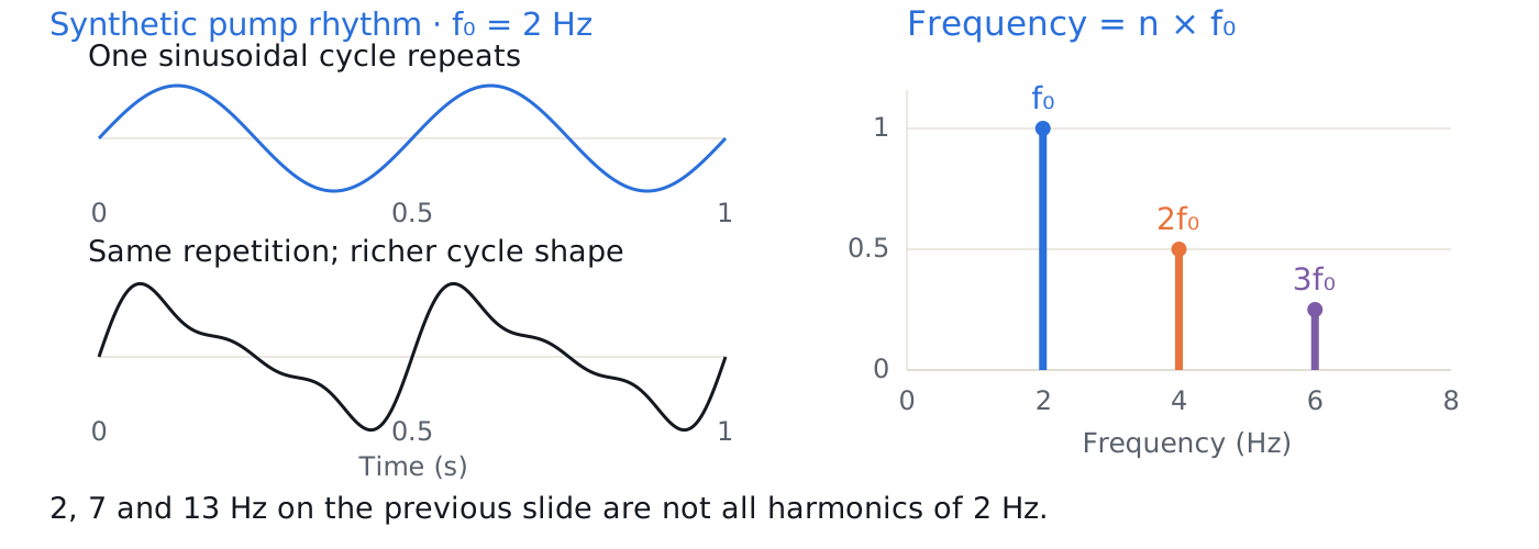
Harmonics are integer multiples of a fundamental: fₙ = n f₀.

A synthetic 2 Hz pump cycle gains spectral peaks at 4 and 6 Hz when its shape changes within each cycle.

Worked example

A Fourier coefficient measures agreement

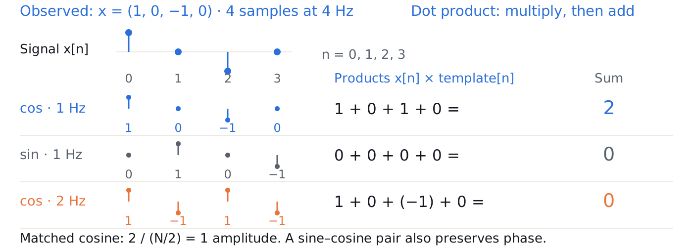
Multiply samples by a candidate wave, then add: matching structure survives the sum.

Four samples and three templates give dot products 2, 0 and 0, showing matched agreement and positive–negative cancellation.

Transform versus summary

Core idea

Keep the phase

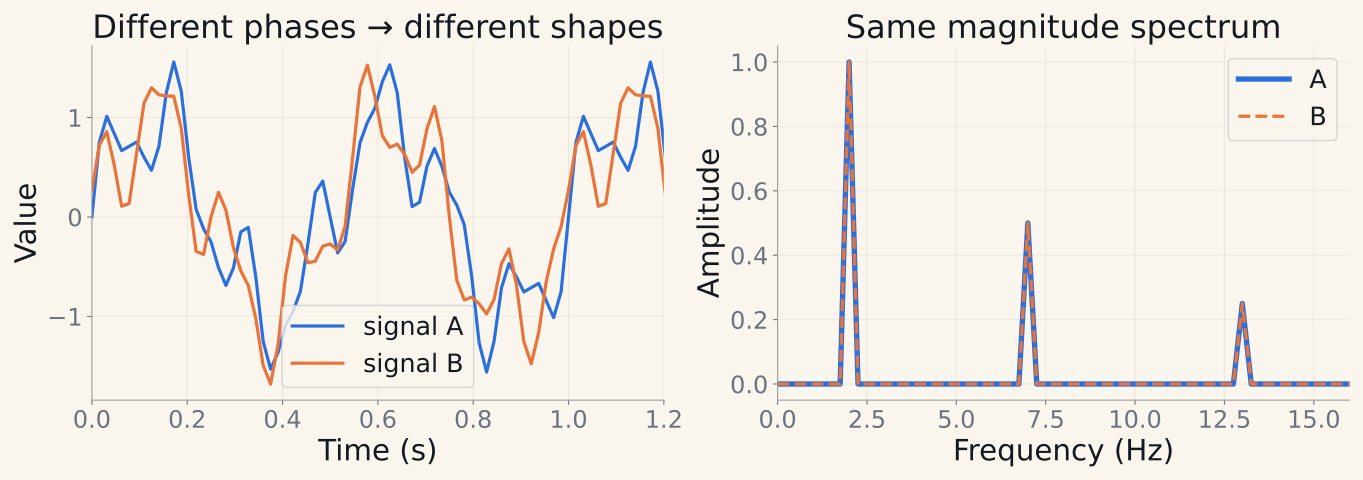
Full FFT coefficients ↔ original samples. Magnitude alone discards phase.

Two signals with the same Fourier magnitudes but different phases have different waveforms. — Constructed teaching signal · fixed seed 20261029

Worked example

Put units on the frequency axis

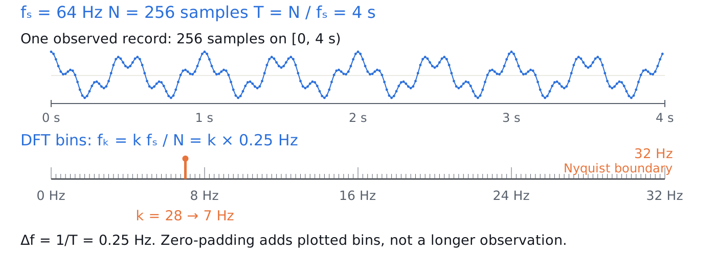
Bin spacing comes from observation duration; zero-padding only samples the spectrum more densely.

A 256-sample, four-second record at 64 Hz maps Fourier bin 28 to 7 Hz, with 0.25 Hz spacing and a 32 Hz Nyquist boundary.

Aliasing is an information limit

Worked example

Can these samples tell two waves apart?

At 10 Hz sampling, these sample values are identical. Sampling faster can distinguish them.

A 2 Hz and an 8 Hz cosine produce identical samples when sampled at 10 Hz. — Constructed teaching signal · fixed seed 20261029

Localize the rhythm

Worked example

When did the frequency change?

A time reversal preserves FFT magnitudes. A spectrogram exposes the order of events.

Opposite frequency-change orders have different spectrograms. — Constructed teaching signal · fixed seed 20261029

The STFT tradeoff

Core idea

Choose a window. Choose a resolution.

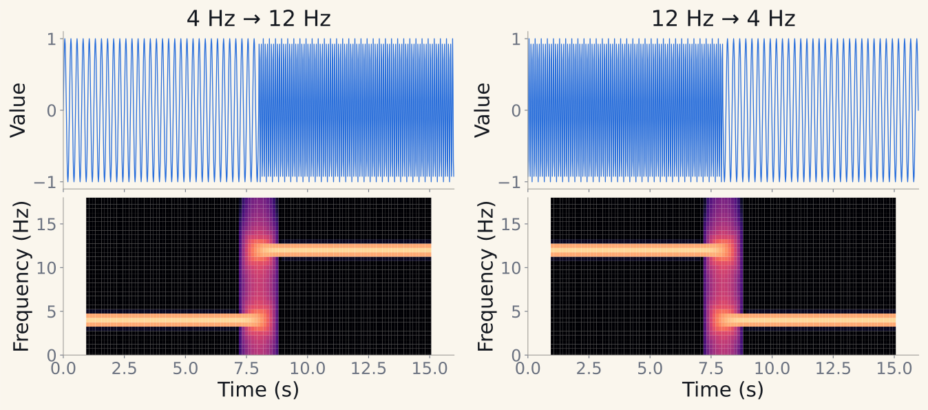
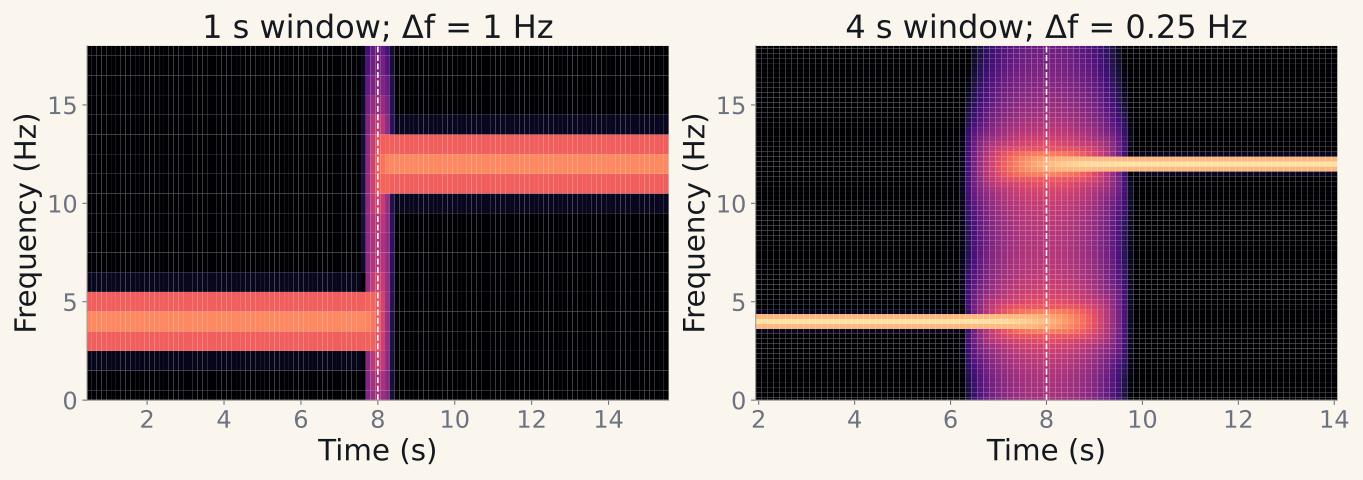
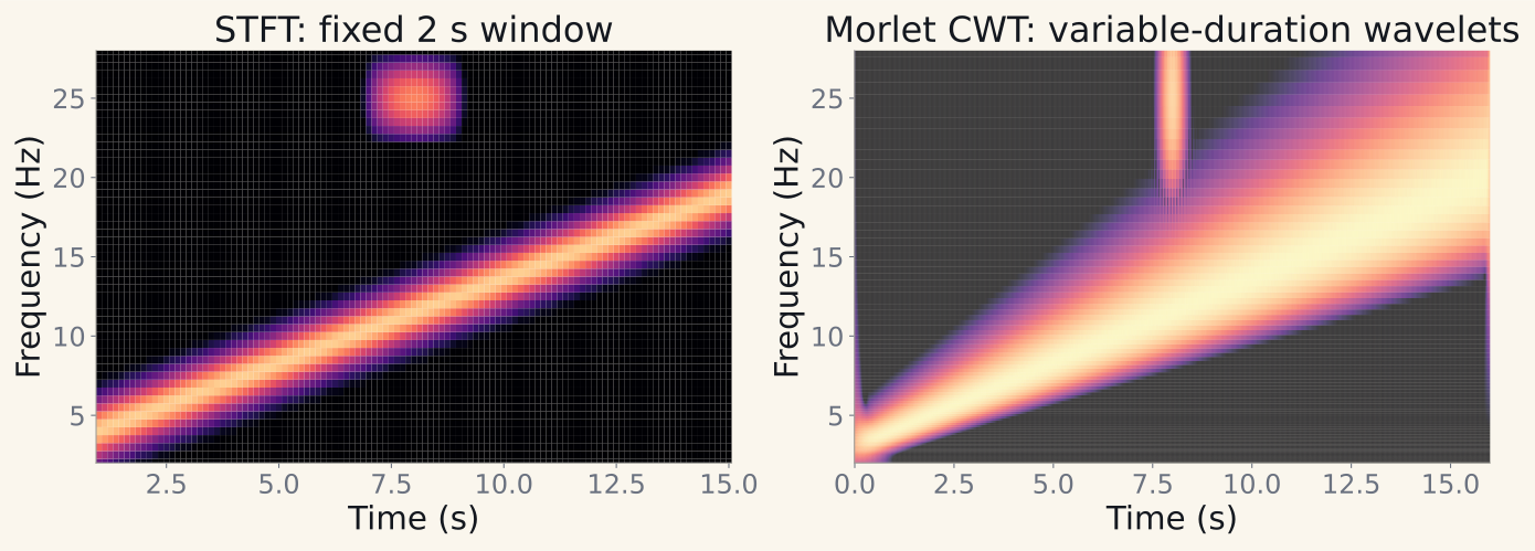
Short windows localize transitions. Long windows separate close frequencies.

Spectrograms of the same changing-frequency signal with one-second and four-second Hann windows. — Constructed teaching signal · fixed seed 20261029

Worked example

A wavelet stretches with the question

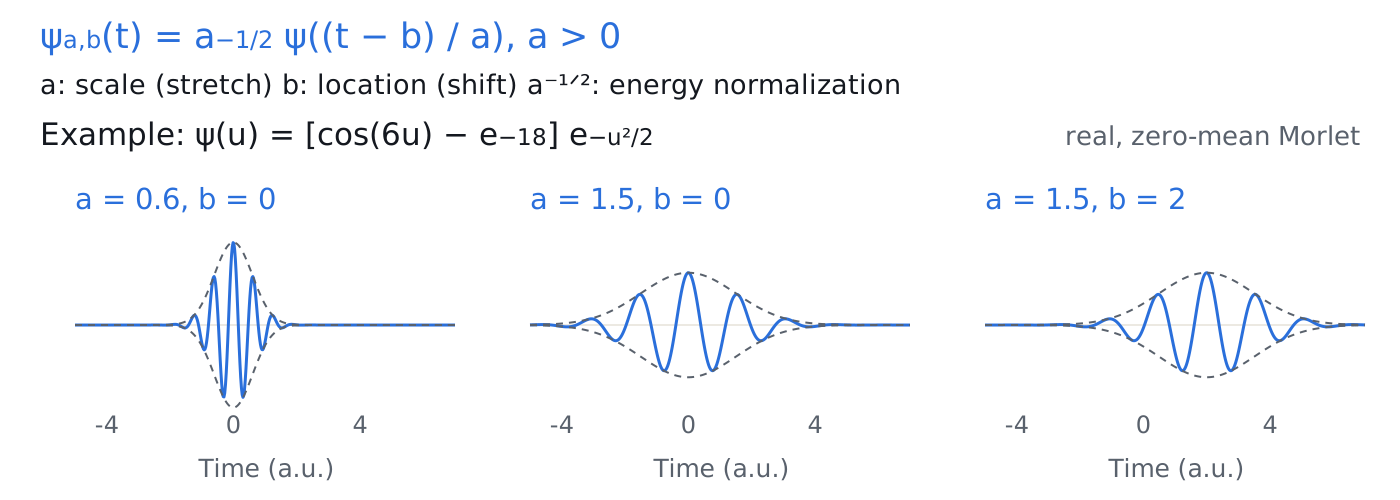
Scale changes duration and frequency; translation chooses where the probe looks.

A corrected real Morlet function is stretched from scale 0.6 to 1.5, then shifted to location 2.

Worked example

Choose or design the wavelet for the event

Different probes emphasize different shapes; their mathematical constraints still matter.

Haar, Mexican hat and Morlet have different waveforms. Changing the Morlet carrier changes the number of oscillations.

The same constructed chirp and burst

Worked example

STFT and CWT ask different local questions

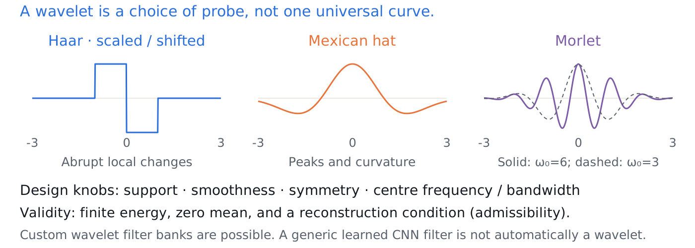
STFT uses one duration. CWT uses multiple scales. Choose the representation for the event.

STFT and a Morlet continuous-wavelet scalogram on the same synthetic frequency sweep and brief high-frequency burst. — Constructed teaching signal · fixed seed 20261029

Turn history into a vector

Core idea

A window becomes one training example

For an anomaly decision after observing x[t], every feature must use times ≤ t.

The simplest learned temporal input

Worked example

Lags preserve recent history

Decision time	x[t]	x[t−1]	x[t−2]	Optional target
2	4	2	1	x[3] = 3
3	3	4	2	x[4] = 5
4	5	3	4	not observed yet

Lag features let a tabular model use order. The target determines the alignment.

Pump investigation 4/8 · Is a change the same as a fault?

Worked example

Change is not the same as state

A sustained level anomaly remains visible in raw level but only its boundaries stand out in first differences or within-window standardization. — Constructed teaching signal · fixed seed 20261029

Noise reduction versus adaptation

Worked example

Smoothing costs response time

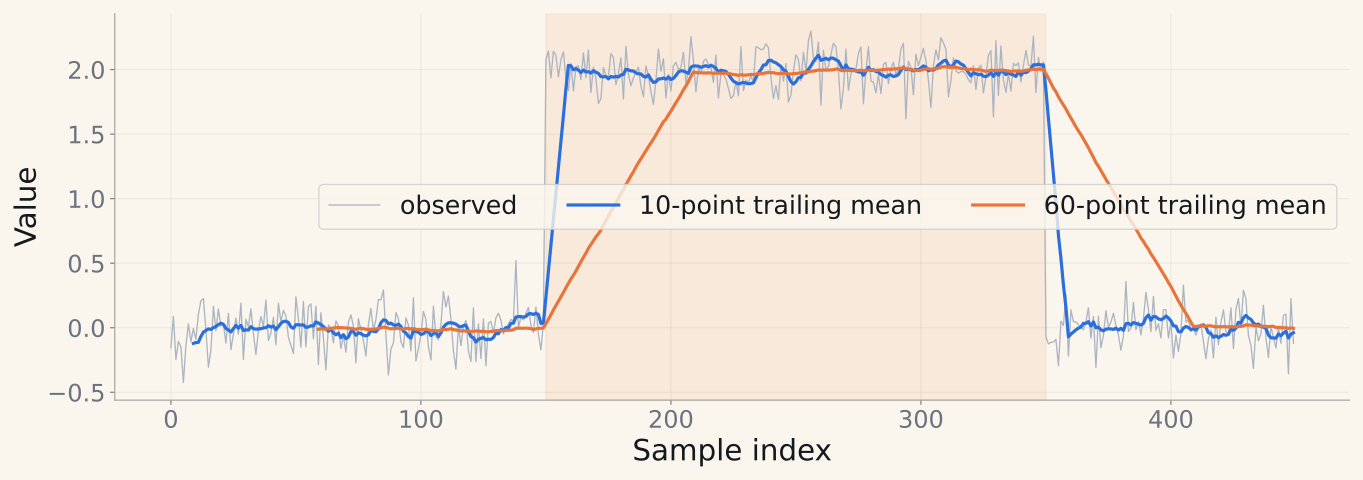
Trailing mean / EWMA: more stable estimates, slower transitions, possible adaptation to a fault.

Ten-point and sixty-point trailing averages respond at different speeds to a sustained shift. — Constructed teaching signal · fixed seed 20261029

Level · spread · extremes

Reference detail

Summaries choose what survives

Family	Examples	Useful for	What it can hide
Level	Mean, median	Persistent offsets	Short transients
Spread	Std, MAD, IQR	Volatility, noisy states	Mean changes
Energy	RMS	Amplitude/energy summaries	Phase and waveform
Extremes	Min/max, quantiles	Spikes, tails, operating limits	Order inside the window
Dynamics	Difference, slope, ACF	Transitions and persistence	Absolute level

Use the frequency content you actually recorded

Reference detail

Spectral features summarize rhythm

A spectrum of SKAB RMS describes modulation of RMS — not the missing raw vibration spectrum.

Fourier / STFT features

Peak frequency and band power

Spectral centroid or entropy

Pick the bands and window from the domain.

Wavelet features

Energy across selected scales

Transient coefficient peaks

State the wavelet, scale mapping, and edge policy.

A multivariate anomaly

Core idea

Relationships can fail first

Useful features: channel differences, rolling covariance, or distance from a learned normal subspace.

Normally two synthetic sensor variables agree; an abnormal relation reverses their dependence while each marginal distribution remains similar. — Constructed teaching signal · fixed seed 20261029

A reproducible feature pipeline

Core idea

Fit transformations on the past

Build and evaluate a feature pipeline using only information available at deployment.

Check the clock
units · gaps · mask→Build causal features
raw + chosen history→Fit on train
scaler · detector

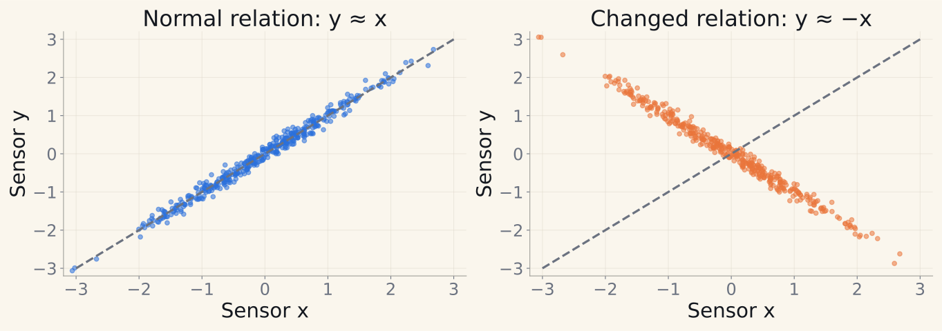
Choose invariances deliberately: per-window centering can erase the very fault we want to detect.

The same history can answer different questions

Core idea

Five tasks. Five different outputs.

Task	Output	Example
Classification	One label per window	Movement type from IMU / EEG epoch
Forecasting	Future values / distributions	Next-hour demand
Anomaly detection	Score, then abnormal-state decision	Pump monitoring
Segmentation	State label at each time	Walking → standing → sitting
Imputation	Values at missing positions	Lost telemetry blocks

A small model can expose a wrong experiment

Core idea

Start with a task-shaped baseline

Task	First comparison	Next step
Classification	Statistics + logistic regression	ROCKET / EEGNet
Forecasting	Last value / seasonal naïve	Lag regression / foundation model
Anomaly detection	Robust normal-state distance	PCA / Isolation Forest / score ensemble
Segmentation	Thresholds / HMM	Temporal CNN; change-point methods
Imputation	Last value / interpolation	Kalman model / learned imputation

One boundary, two legitimate tasks

Core idea

What was available at decision time?

Causality depends on the decision time, not on the model’s name.

Forecast issued before x[t]

x[≤t−1] → x̂[t]

Use the error only after x[t] arrives.

State decision after x[t]

x[≤t] → s[t]

A trailing statistic may include the current observation.

Evaluation is part of the model

Core idea

Overlapping windows are not independent

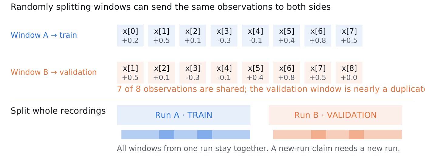
These length-eight windows share seven observations. A new-run evaluation holds out whole recordings.

Evaluation is part of the model

Worked example

Roll the forecast origin forward

Expanding windows retain all earlier data; rolling windows keep a fixed recent history.

Evaluation is part of the model

Core idea

Hold out the identity you expect to meet

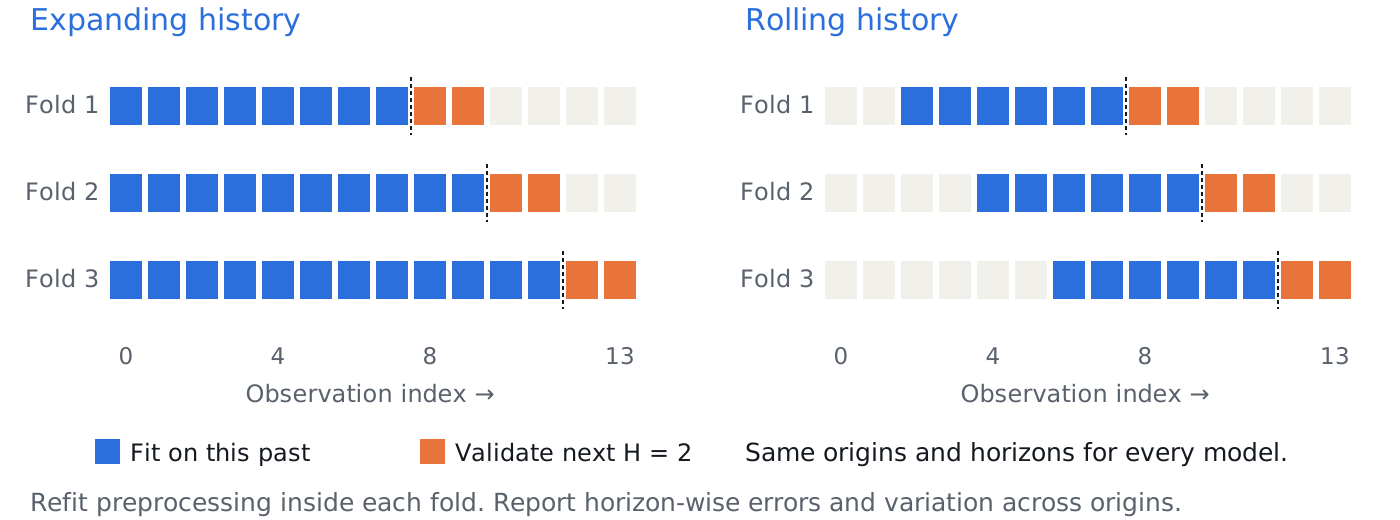
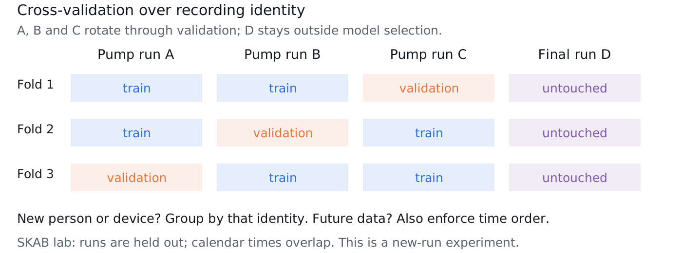
Time splits test the future; group splits test new runs, people or devices. Some deployments require both.

Evaluation is part of the model

Core idea

Guard the information boundary

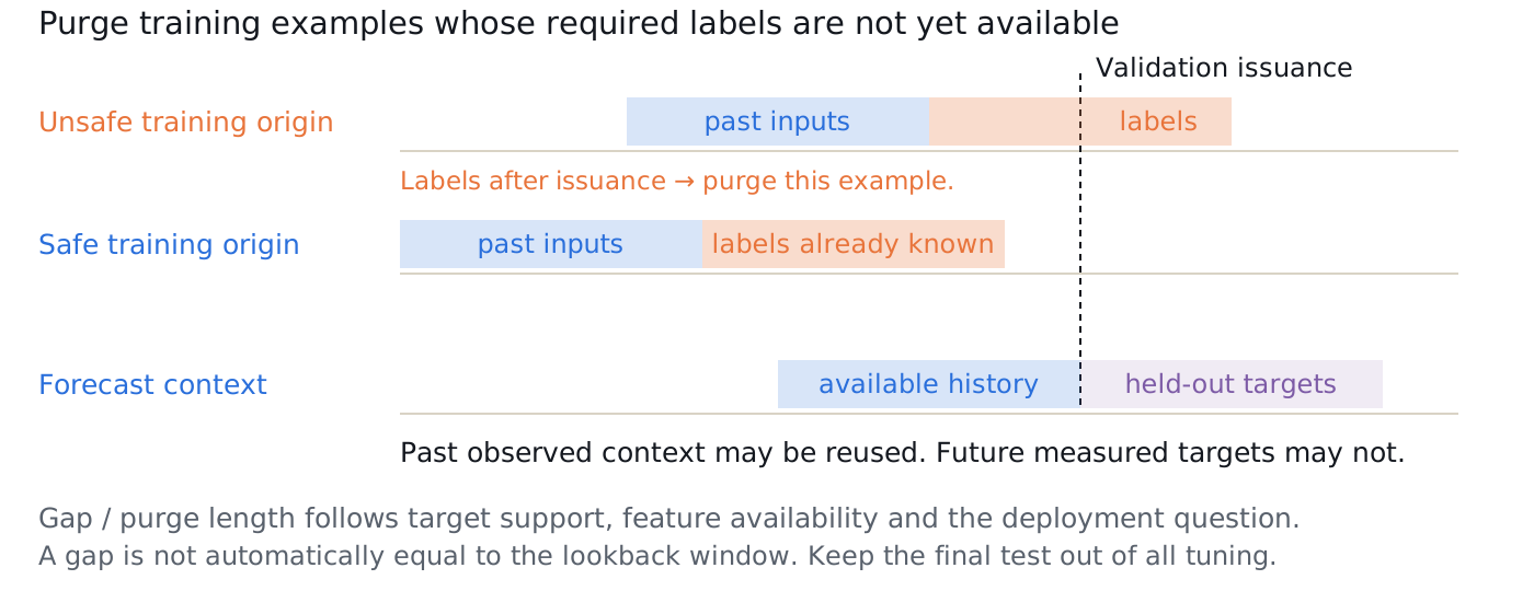
Choose the gap from what each training example needs to know; preserve legitimately available forecasting history.

Transfer check · Choose → explain → reveal

Core idea

Choose the split for a new person and a later date

Transfer check · Choose → explain → reveal

Core idea

Choose a feature for a new fault

Follow the mechanisms

Reference detail

Sources, credits, and reproducible controls

Read and explore

Hyndman & Athanasopoulos: Forecasting: Principles and Practice

3Blue1Brown: Fourier transform intuition

PyWavelets: continuous wavelets, scale and frequency

Data and illustration

Katser & Kozitsin: SKAB

Serega artwork reused from Albert Nasybullin’s Deep Learning for Search course.

Scientific control plots are computed; synthetic plots are labeled explicitly.

Clickable sources, credits and figure provenance.

A robot

A person

A service

Weak stationarity

Useful diagnostics

Time

Frequency

Time–frequency

Fourier / STFT features

Wavelet features

Forecast issued before x[t]

State decision after x[t]

Read and explore

Data and illustration

Keyboard