Can attention tell who bites whom? · Exact examination statement · 1/2
Consider one self-attention layer on three token embeddings . There are no positional features, masks or dropout. Queries and keys have dimension . The same matrices are used at every position: Compare A: “dog bites man” with B: “man bites dog”. Each word has a fixed embedding, so B exchanges and keeps . A classifier receives only , the contextual representation of “bites”.
Variant 1, Task 30. Questions
Can attention tell who bites whom? · Exact examination statement · 2/2
(a) Express B’s three weights for query 2 in terms of A’s weights. Use this to prove that the classifier receives the same vector in A and B.
(b) Is the entire ordered output also necessarily unchanged? Give its exact relation to A’s output and justify it.
(c) Now replace each input by , where is a fixed vector attached to position . Explain precisely why the previous permutation argument need no longer hold when . Does this guarantee that every choice of distinguishes the sentences? Justify.
Follow the words through the swap
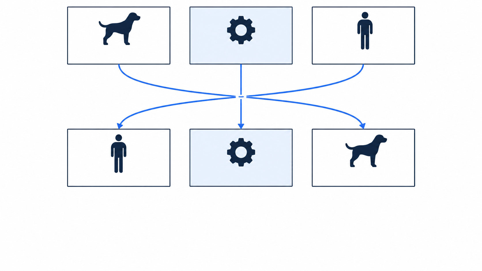
Variant 1 · A word keeps its embedding when its slot changes
dog · bites · man ·
man · bites · dog ·
The middle query stays fixed; keys and values move together.
Can attention tell who bites whom?
Variant 1 · Fixed word embeddings · Shared weights · No positions, masks or dropout
Sentence
Position 1
Position 2
Position 3
A
dog
bites
man
B
man
bites
dog
Vocabulary [dog, bites, man]: , , . Word identity stays fixed when its slot changes. The classifier reads only .
The middle word stays in place: .
Keys and values exchange slots 1 and 3 together.
The middle representation
Variant 1(a) · A has weights
Illustration with one-hot values: move as pairs. Their sum stays .
Swapping the keys reorders the denominator’s three terms. Its sum stays fixed.
A deterministic classifier of receives the same vector.
Outputs follow the words
Variant 1(b) · Rows are query slots; columns are key/value slots
Stack token transposes as rows: , , , .
Both query rows and key columns move. Row denominators keep the same terms:
The sequence is equivariant; the selected middle row is unchanged.
Position supplies additional information
Variant 1(c) · Replace each word input by , with
A’s endpoints
B’s endpoints
Augmented inputs
Position vectors stay attached to slots when words move.
Their difference is when . The swap proof no longer guarantees the output relation.
A counterexample to a guarantee: makes every output zero.
Position can enable a distinction; learned weights must use it.
Variant 2, Task 30.
Why more models can stop helping · Exact examination statement · 1/2
At a fixed input , repeated random training runs produce predictions , where . For a fixed target value , assume The ensemble prediction is . All expectations concern randomness in training, not different inputs. You may use and .
Variant 2, Task 30. Questions
Why more models can stop helping · Exact examination statement · 2/2
(a) Expand the square in the variance definition to derive . Show how many diagonal and off-diagonal terms occur; do not quote a memorized ensemble formula.
(b) By adding and subtracting , derive . Find its limit as and explain which two obstacles cannot be removed merely by increasing .
(c) Suppose . Can any finite make the ensemble variance at most ? Explain. What does the formula say when ?
Averaging random predictions
Variant 2 · Fixed input and target · Randomness comes from training
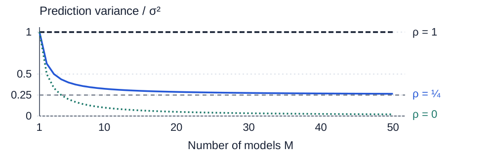
Fixed target → common center → predictions . Averaging changes their spread, while the common center stays fixed.
Center each prediction: .
Here is common prediction bias and is prediction variance across training runs.
Counting covariance terms
Variant 2(a) · Expand the square before simplifying
Example:
σ²
ρσ²
ρσ²
ρσ²
ρσ²
σ²
ρσ²
ρσ²
ρσ²
ρσ²
σ²
ρσ²
ρσ²
ρσ²
ρσ²
σ²
4 diagonal + 12 ordered off-diagonal terms
Correlated fluctuations survive averaging.
Bias and variance in prediction error
Variant 2(b) · What remains after averaging?
Error budget: common bias² + shared fluctuation + averaged fluctuation.
Can a finite ensemble reach the floor?
Variant 2(c) · Set
At , the variance stays for every .
Variant 3, Task 30.
Build a lower bound from a weighted average · Exact examination statement · 1/2
Fix an observation . A latent variable takes values . The model specifies strictly positive numbers , and . Choose any probabilities with . Define You may use the strict concavity of the natural logarithm: for , with equality exactly when all are equal.
Variant 3, Task 30. Questions
Build a lower bound from a weighted average · Exact examination statement · 2/2
(a) Rewrite as a -weighted average and prove . Find the unique that gives equality and identify it probabilistically.
(b) Let and define . Show by expansion that . What does part (a) tell you about the sign of ?
(c) If , rewrite as an expected log-likelihood minus , using the same definition of . Explain the two terms in one sentence. This bound is called the ELBO.
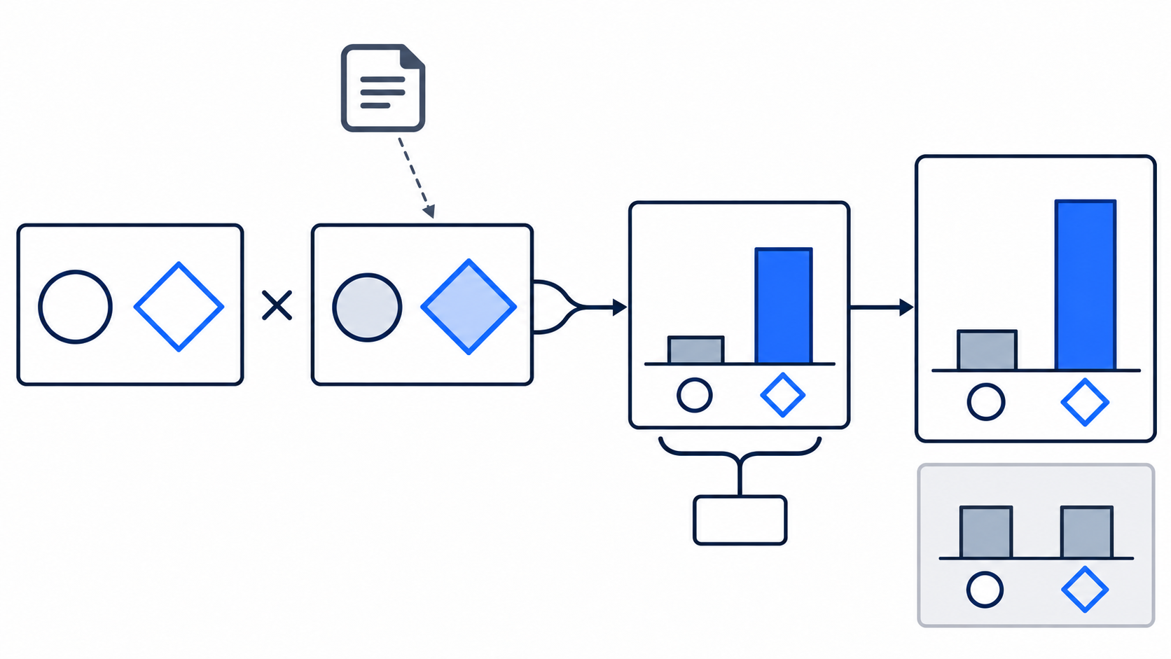
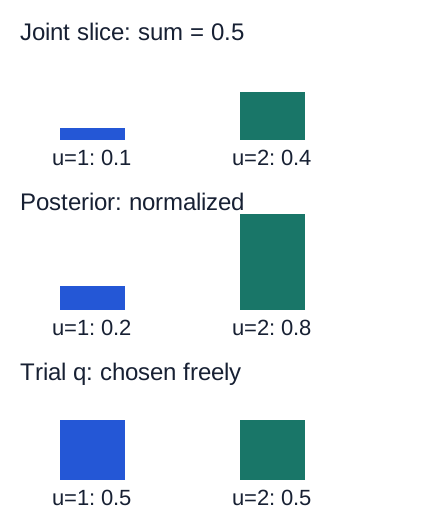
Evidence is a scalar. The posterior is a distribution over hidden states.
Evidence is a sum over hidden states
Variant 3 · Fix an observation · Latent state
Joint masses → sum → normalize to posterior .
Choose , :
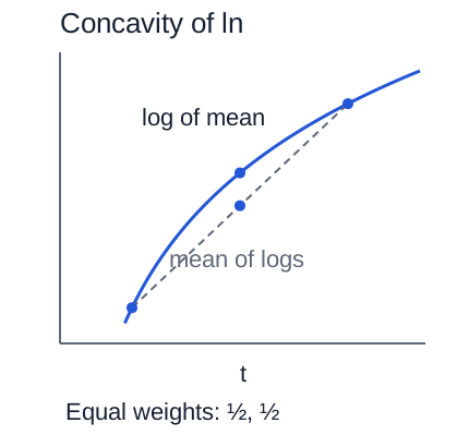
Supplied tool: concavity of the natural logarithm
Equality holds exactly when all are equal.
A weighted average inside the logarithm
Variant 3(a) · How can the supplied inequality apply to the evidence?
Set . The weights sum to one.
Every admissible gives a lower bound on log evidence.
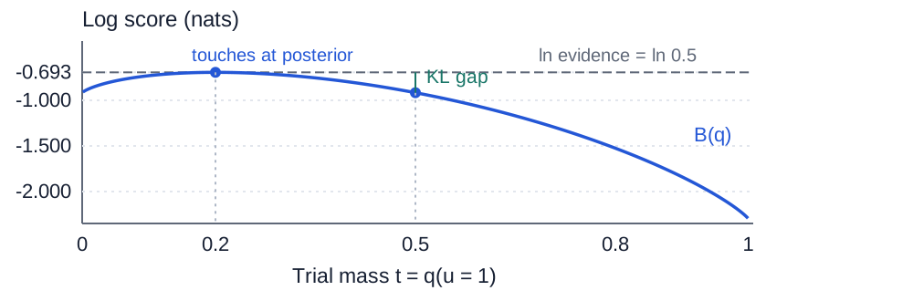
When does the bound touch the evidence?
Variant 3(a) · Use the equality condition and normalization
The unique equality distribution is the exact posterior.
The model is fixed. Varying changes the bound; log evidence stays fixed.
The gap is a posterior KL
Variant 3(b) · Define and
Fixed log evidence = chosen bound + nonnegative inference gap. The gap compares with the posterior, not the prior.
Since ,
The posterior KL measures how far the bound falls below log evidence.
Two KLs, two different questions
Variant 3(c) · Prior · Trial · Posterior
Posterior KL: how much does inference miss? Prior KL: what does the code cost?
Course notation: is the ELBO, maximized during fitting.
An exact posterior closes the gap; it need not equal the prior.
An exact two-state check
Additional example · Joint masses · Evidence · Posterior
: .
; gap .
: both joint-to- ratios equal , so the gap is zero.
Variant 4, Task 30.
Good reconstruction or a useful latent variable? · Exact examination statement · 1/2
Let both the observation and latent variable be binary. The prior is . Compare two complete models:
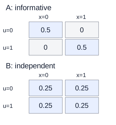
Model A: and ; its encoder assigns .
Model B: for either ; its encoder assigns .
For the observation , define the reconstruction score and latent cost The training score is , which is maximized. Zero-probability encoder states are omitted from these sums. Natural logarithms are used. You may use and .
Variant 4, Task 30. Questions
Good reconstruction or a useful latent variable? · Exact examination statement · 2/2
(a) Compute and by summing over . Can likelihood of this observation distinguish the two models?
(b) Compute , and for each model. Explain why the model with better reconstruction does not obtain a better total score here.
(c) Use Bayes’ rule to find and . Which latent variable carries information about , and which model ignores it? Explain why equal likelihood need not imply equally informative latent representations.