Introduction to Machine Learning
Experience, tasks, measures—and the roots of MSE
By the end of this lecture
You should be able to:
- formulate a learning problem through experience, a task, a performance measure, and its scope;
- distinguish a model, a training loss, and an evaluation metric;
- formulate linear regression as a learning problem;
- derive MSE from Gaussian maximum likelihood;
- explain why input-dependent noise changes the loss.
What this course should change
Not only:
I can call a library and train a model.
But:
I can state what the model learns, from what evidence, under which assumptions—and how we know whether it works.
One week, one learning loop
Before: a short question reveals what needs attention.
Lecture: we find the few ideas from which the methods grow.
Tutorial: we turn the ideas into mathematics and code.
Laboratory: we test them on a problem that can fail.
After: a short question checks what changed.
The syllabus is the source of truth
The course currently offers up to 112 points across semester activities and the midterm.
For the current allocation, grade ranges, and policy status, use the course syllabus.
Slides explain ideas. The syllabus governs course logistics.
Machine learning sits inside a larger map
“When I use a word … it means just what I choose it to mean—neither more nor less.”
— Humpty Dumpty, Lewis Carroll
Artificial intelligence is the broader ambition.
Machine learning improves performance through experience.
Deep learning is a family of machine-learning methods based on learned multilayer representations.
Mitchell gives us \(E\), \(T\), and \(P\)
A program learns from:
\[ \boxed{\text{Experience }E\quad +\quad \text{Task }T\quad +\quad \text{Performance measure }P} \]
when its performance at tasks in \(T\), as measured by \(P\), improves with experience \(E\).
This course adds scope \(S\)
Scope \(S\) states where we expect the performance claim to hold: which population, period, environment, and operating conditions.
\[ E + T + P \quad\Longrightarrow\quad \text{a measured result} \]
\[ E + T + P + S \quad\Longrightarrow\quad \text{an interpretable claim} \]
The four parts define a learning claim
| Part | House-price example |
|---|---|
| Experience \(E\) | Moscow apartment sales from 2024–2025 |
| Task \(T\) | Predict sale price from available features |
| Performance \(P\) | Mean absolute error on held-out sales |
| Scope \(S\) | Similar Moscow apartments under comparable market conditions |
The algorithm is a candidate solution—not the learning problem itself.
Physics and learning answer different questions
Mechanistic route
Physical laws + initial conditions
\[ \Downarrow \]
Predicted trajectory
Learning route
Observed examples + assumptions
\[ \Downarrow \]
Fitted predictive rule
Experience is broader than a labelled table
- Supervised: observed input–target pairs \((x_i,y_i)\).
- Unsupervised: observations \(x_i\), without supplied targets.
- Self-supervised: supervision constructed from the observations.
- Reinforcement: trajectories of states, actions, and rewards.
Experience is the information allowed to change the model.
Representation determines what the model can see
| Raw object | Possible representation |
|---|---|
| apartment | a fixed vector of measured attributes |
| image | a height × width × channel tensor |
| sentence | a sequence of tokens or embeddings |
| sensor stream | a time-ordered sequence of measurements |
The same real object can support several representations—and different learning problems.
Data is evidence, not reality
A dataset is finite and selective. It may contain:
- measurement noise and label errors;
- missing or imperfect variables;
- sampling bias and dependence;
- conditions that later change.
Box’s point was that models inevitably simplify reality; the useful question is whether their discrepancies matter for the intended purpose.
Most of the learning system surrounds the model
\[ \text{question} \rightarrow \text{data} \rightarrow \text{split} \rightarrow \text{preprocessing} \rightarrow \text{fit} \rightarrow \text{evaluate} \rightarrow \text{claim} \]
Leakage, sampling, preprocessing, and evaluation design can matter more than changing the model family.
A task specifies the required output
It does not specify the architecture.
The same task may be approached with a linear model, a tree, a neural network, or a pretrained model.
Name the output and its structure before choosing the machinery that produces it.
Tasks differ through their inputs and outputs
| Task | Input | Output | Example |
|---|---|---|---|
| regression | feature vector | continuous value | apartment → price |
| classification | text, image, or vector | discrete class | review → sentiment |
| segmentation | image | class at each pixel | street scene → region labels |
| depth estimation | image | value at each pixel | scene → distance map |
| captioning | image | text sequence | image → description |
| generation | prompt or context | new structured sample | prompt → image |
| control | state or history | action | board position → move |
Learning settings and tasks are different axes
Learning setting: where the experience or feedback comes from.
Task: what the fitted system must produce.
For example, classification can use supervised labels, self-supervised pretraining, or feedback gathered through interaction.
A performance measure makes learning falsifiable
The measure \(P\) answers:
What observable change would convince us that the system became better at the task?
Without a declared measure, “the model learns” is only a story.
Different tasks demand different measures
| Task | Possible measure \(P\) |
|---|---|
| house-price regression | RMSE or MAE |
| disease detection | sensitivity at fixed specificity |
| image segmentation | IoU or Dice |
| ranking | NDCG |
| control | expected cumulative return |
The choice expresses which errors matter.
Performance measure and loss are not synonyms
- Performance measure: judges the fitted system on validation or test data.
- Loss: supplies a numerical objective for fitting model parameters.
They may coincide, but often do not. Accuracy, Dice, and task success can be awkward to optimize directly.
Start with the claim
This fitted model will perform well on future cases from scope \(S\).
To examine that claim, we need data that did not determine the fitted model.
\[ \widehat R_{\mathrm{test}}(f) =\frac{1}{n_{\mathrm{test}}} \sum_{i=1}^{n_{\mathrm{test}}} L\!\left(y_i,f(x_i)\right) \]
Training and evaluation play different roles
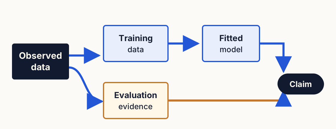
A minimal validation split enforces separation
This demonstrates separation—not a complete evaluation strategy.
The same score can support different conclusions
More credible evidence
- split fixed before fitting;
- preprocessing fitted on training data;
- metric matches the task;
- variation is reported.
Misleading evidence
- test data guides choices;
- features use future information;
- metric hides costly errors;
- only the best run is shown.
Before choosing an algorithm
Write down:
- experience \(E\);
- task \(T\);
- performance measure \(P\);
- target scope \(S\);
- assumptions and evaluation protocol.
Then ask what could make the resulting estimate optimistic.
Our first concrete task is regression
Given examples
\[ \mathcal D=\{(x_i,y_i)\}_{i=1}^{n}, \]
learn a function that predicts a continuous target \(y\) from input \(x\).
Today we will ask where the familiar squared-error objective comes from.
The simplest model is linear in its parameters
For one feature,
\[ f_{\theta}(x)=\theta_0+\theta_1x. \]
For \(d\) features,
\[ f_{\boldsymbol\theta}(\mathbf x) =\theta_0+\mathbf x^{\mathsf T}\boldsymbol\theta. \]
“Linear” refers to the parameters—not necessarily to the original raw features.
Residuals compare observations with predictions
For example \(i\),
\[ \hat y_i=f_{\theta}(x_i), \qquad r_i=y_i-\hat y_i. \]
The sign tells us the direction of the error; the magnitude tells us how far the prediction missed.
MSE turns residuals into one objective
\[ \operatorname{MSE}(\theta) =\frac{1}{n}\sum_{i=1}^{n} \left[y_i-f_{\theta}(x_i)\right]^2. \]
Squaring prevents positive and negative residuals from cancelling and penalizes large residuals strongly.
But why should this particular objective be principled?
Optimization searches over parameter values
Gradient descent follows local slope information:
\[ \theta^{(k+1)} =\theta^{(k)} -\eta\,\nabla_{\theta}\operatorname{MSE}\!\left(\theta^{(k)}\right). \]
The learning rate \(\eta\) controls the step size—not the direction supplied by the gradient.
A landscape is useful—but only as an analogy
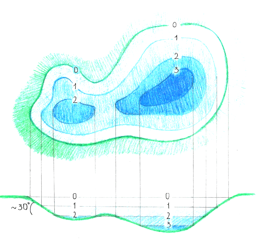
The gradient provides a local downhill direction. It does not guarantee that every optimization problem reaches the globally best destination.
A point prediction hides an observation model
A prediction \(f_{\theta}(x)\) gives one value.
Observed outcomes still vary around that value, so we can instead specify
\[ p(y\mid x;\theta), \]
a conditional distribution of plausible outputs for a given input.
Variables and observations need different notation
- \(X,Y\): random variables;
- \(x_i,y_i\): observed values in example \(i\);
- \(p_{Y\mid X}(y\mid x)\): the conditional density of \(Y\), evaluated at \(y\), after observing \(X=x\).
We usually shorten the final expression to \(p(y\mid x)\) when the variables are clear.
Prediction needs \(p(y\mid x)\), not only \(p(y)\)
The prediction problem asks:
Which outputs are plausible for this input?
The marginal distribution \(p(y)\) ignores \(x\). The conditional distribution \(p(y\mid x)\) uses it.
Why not write \(p(f)\)?
In ordinary regression, \(f_{\theta}\) is a deterministic mapping. It can produce parameters of a distribution:
\[ x\xrightarrow{f_{\theta}} \bigl(\mu(x),\sigma(x)\bigr) \quad\Longrightarrow\quad p(y\mid x;\theta). \]
A distribution over functions is possible in Bayesian modelling, but that is a different modelling choice.
Likelihood evaluates the observed data under the model
For fixed observed data \(\mathcal D\), the likelihood is a function of the parameters:
\[ \mathcal L(\theta;\mathcal D) =p(\mathbf y\mid\mathbf X;\theta). \]
Maximum likelihood chooses parameters under which the observed targets are comparatively probable.
Conditional independence creates a product
If targets are conditionally independent given their inputs and parameters,
\[ p(\mathbf y\mid\mathbf X;\theta) =\prod_{i=1}^{n}p(y_i\mid x_i;\theta). \]
This factorization is what the derivation needs. Assuming complete examples are IID is a common, stronger sampling assumption.
The logarithm turns the product into a sum
\[ \hat\theta_{\mathrm{MLE}} =\arg\max_{\theta} \prod_{i=1}^{n}p(y_i\mid x_i;\theta) \]
is equivalent to
\[ \hat\theta_{\mathrm{MLE}} =\arg\min_{\theta} \left[-\sum_{i=1}^{n}\log p(y_i\mid x_i;\theta)\right]. \]
Homoscedastic Gaussian regression assumes constant noise
Assume
\[ Y_i\mid X_i=x_i \sim\operatorname{Normal}\!\left(f_{\theta}(x_i),\sigma^2\right), \]
where the same variance \(\sigma^2\) applies to every input.
The model predicts the conditional mean; \(\sigma^2\) describes one shared noise level.
Gaussian maximum likelihood becomes squared error
For one observation,
\[ -\log p(y_i\mid x_i;\theta) =\frac{1}{2}\log(2\pi\sigma^2) +\frac{\left[y_i-f_{\theta}(x_i)\right]^2}{2\sigma^2}. \]
For fixed \(\sigma^2\), constants and positive scale factors do not change the minimizer.
\[ \boxed{\text{Gaussian MLE for the mean}\iff\text{minimize MSE}} \]
Unknown shared variance does not change the fitted mean
Joint maximum likelihood gives
\[ \hat\theta =\arg\min_{\theta}\sum_i \left[y_i-f_{\theta}(x_i)\right]^2, \]
followed by
\[ \hat\sigma^2_{\mathrm{MLE}} =\frac{1}{n}\sum_i \left[y_i-f_{\hat\theta}(x_i)\right]^2. \]
The denominator \(n\) is the MLE result; unbiased variance estimation is a different question.
MSE carries modelling assumptions
The Gaussian-likelihood derivation encodes:
- conditional mean \(f_{\theta}(x)\);
- conditionally independent residuals;
- one constant conditional variance;
- a quadratic penalty that emphasizes large residuals.
This is one principled origin of MSE—not its only justification. Under finite second moments, expected squared error targets the conditional mean.
Heteroscedastic regression makes noise input-dependent
Now assume
\[ Y_i\mid X_i=x_i \sim\operatorname{Normal}\!\left( \mu_{\theta}(x_i), \sigma_{\theta}^{2}(x_i) \right). \]
The model predicts both a conditional mean and an input-dependent variance.
The heteroscedastic loss balances fit and uncertainty
Let \(s_{\theta}(x)=\log\sigma_{\theta}^{2}(x)\). Ignoring a constant,
\[ \ell_i(\theta) =\frac{1}{2}\left[ s_{\theta}(x_i) +e^{-s_{\theta}(x_i)} \left(y_i-\mu_{\theta}(x_i)\right)^2 \right]. \]
The residual can be attenuated by uncertainty; the log-variance term prevents every predicted variance from growing without bound.
The noise model changes what can be predicted
| Homoscedastic | Heteroscedastic | |
|---|---|---|
| Mean | \(\mu_{\theta}(x)\) | \(\mu_{\theta}(x)\) |
| Variance | one \(\sigma^2\) | \(\sigma_{\theta}^2(x)\) |
| Loss | MSE, up to constants and scale | Gaussian NLL |
| Output | mean + optional global noise | mean + input-dependent aleatoric uncertainty |
The second model answers a richer question, but it also has more ways to be wrong.
The roots found today
- Mitchell defines learning through \(E\), \(T\), and \(P\); this course adds target scope \(S\).
- A task defines the output, while experience defines what may change the model.
- A loss fits parameters; a performance measure judges the resulting system.
- Gaussian maximum likelihood with constant variance leads to MSE.
- Input-dependent variance leads to a different loss and a richer prediction.
Can you now answer these?
- Identify \(E\), \(T\), \(P\), and \(S\) for one application.
- Why do we model \(p(y\mid x)\) rather than only \(p(y)\)?
- Which assumptions connect Gaussian maximum likelihood to MSE?
- Why are training loss and evaluation metric different concepts?
- What prevents a heteroscedastic model from predicting infinite variance?
References
- Bishop, C. M. (2006). Pattern Recognition and Machine Learning. Springer.
- Box, G. E. P. (1976). Science and statistics. JASA, 71(356), 791–799. https://doi.org/10.1080/01621459.1976.10480949
- Carroll, L. (1871). Through the Looking-Glass. Chapter VI. https://www.gutenberg.org/ebooks/12
- Goodfellow, I., Bengio, Y., & Courville, A. (2016). Deep Learning. MIT Press. https://www.deeplearningbook.org/
- Kendall, A., & Gal, Y. (2017). What uncertainties do we need in Bayesian deep learning for computer vision? NeurIPS 30.
- Mitchell, T. M. (1997). Machine Learning. McGraw-Hill.
- Nix, D. A., & Weigend, A. S. (1994). Estimating the mean and variance of the target probability distribution. ICNN’94, 1, 55–60. https://doi.org/10.1109/ICNN.1994.374138
- Prince, S. J. D. (2023). Understanding Deep Learning. MIT Press. https://udlbook.github.io/udlbook/
← Lectures Introduction to Machine Learning · 01